数据集

In [1]:

1
2
3
4
5
import sys, os
sys.path.append(os.pardir) # 为了导入父目录的文件而进行的设定
import numpy as np
from dataset.mnist import load_mnist # 导入处理数据的脚本
from PIL import Image

In [2]:

1
2
3
def img_show(img):
pil_img = Image.fromarray(np.uint8(img))
pil_img.show()

In [3]:

1
(x_train, t_train), (x_test, t_test) = load_mnist(flatten=True, normalize=False)

In [4]:

1
t_train # 标签数组

Out[4]:

1
array([5, 0, 4, ..., 5, 6, 8], dtype=uint8)

In [5]:

1
x_train.size # 图像

Out[5]:

1
47040000

In [6]:

1
x_train[0].size

Out[6]:

1
784

In [7]:

1
2
3
4
5
img = x_train[0]
label = t_train[0]
print(label) # 5
img_show(img) # 会看到一长条,也就是784 x 1的col vector
5

In [8]:

1
2
3
4
5
print(img.shape)  # (784,)
img = img.reshape(28, 28) # 把图像的形状变为原来的尺寸
print(img.shape) # (28, 28)
(784,)
(28, 28)

In [9]:

1
img_show(img)

神经网络的推理处理

In [10]:

1
import pickle

In [11]:

1
2
3
4
5
6
7
8
9
10
def softmax(a):
c = np.max(a)
exp_a = np.exp(a - c)
sum_exp_a = np.sum(exp_a)
y = exp_a / sum_exp_a

return y

def sigmoid(x):
return 1 / (1+np.exp(-x))

In [12]:

1
2
3
def get_data():
(x_train, t_train), (x_test, t_test) = load_mnist(normalize=True, flatten=True, one_hot_label=False)
return x_test, t_test

In [13]:

1
2
3
4
5
def init_network():
with open("sample_weight.pkl", "rb") as f:
network = pickle.load(f)

return network

In [14]:

1
2
3
4
5
6
7
8
9
10
11
12
def predict(network, x):
W1, W2, W3 = network['W1'], network['W2'], network['W3']
b1, b2, b3 = network['b1'], network['b2'], network['b3']

a1 = np.dot(x, W1) + b1
z1 = sigmoid(a1)
a2 = np.dot(z1, W2) + b2
z2 = sigmoid(a2)
a3 = np.dot(z2, W3) + b3
y = softmax(a3)

return y

In [15]:

1
2
3
4
5
6
7
8
x, t = get_data()
print("矩阵大小是",x.shape)
print("单个图像vector",x[0].shape)
network = init_network()
print("权重矩阵W1", network['W1'].shape)
矩阵大小是 (10000, 784)
单个图像vector (784,)
权重矩阵W1 (784, 50)

In [16]:

1
2
3
4
5
6
7
8
accuracy_cnt = 0
for i in range(len(x)):
y = predict(network, x[i])
p = np.argmax(y)
if p == t[i]:
accuracy_cnt += 1
print('Accuracy:' + str(float(accuracy_cnt) / len(x)))
Accuracy:0.9352

利用批处理实现

In [17]:

1
2
batch_size = 100 # 批数量
accuracy_cnt = 0

In [18]:

1
2
3
4
5
6
7
8
for i in range(0, len(x), batch_size):
x_batch = x[i:i+batch_size]
y_batch = predict(network,x_batch)
p = np.argmax(y_batch, axis = 1) # 沿着第一维方向找到值最大的元素的索引
accuracy_cnt += np.sum(p == t[i:i+batch_size])

print('Accuracy:' + str(float(accuracy_cnt) / len(x)))
Accuracy:0.9352

In [19]:

1
2
3
4
5
# argmax的test
x = np.array([[0.1, 0.8, 0.1], [0.3, 0.1, 0.6], [0.2, 0.5, 0.3], [0.8, 0.1, 0.6]])
y = np.argmax(x, axis = 1)
print(y)
[1 2 1 0]

损失函数

In [1]:

1
2
3
4
5
6
7
8
9
# 均方误差
def mean_squared_error(y, t):
return 0.5 * np.sum((y-t)**2)


# 交叉熵误差
def cross_entropy_error(y, t):
delta = 1e-7 # 保护措施,防止y[i]=0时产生的错误
return -np.sum(t * np.log(y + delta))

mini-batch学习

In [2]:

1
2
3
4
import sys, os
sys.path.append(os.pardir) # 为了导入父目录的文件而进行的设定
import numpy as np
from dataset.mnist import load_mnist # 导入处理数据的脚本

In [3]:

1
(x_train, t_train), (x_test, t_test) = load_mnist(one_hot_label=True, normalize=True) # 注意这里把标签变成0,1vector形式了

In [4]:

1
2
3
4
5
train_size = x_train.shape[0]
batch_size = 10
batch_mask = np.random.choice(train_size, batch_size)
x_batch = x_train[batch_mask]
t_batch = t_train[batch_mask]

In [5]:

1
batch_mask # 随机的10个数

Out[5]:

1
2
array([57147, 30041, 12057, 53543, 31076, 33940, 43334, 28835,  9675,
23190])

In [6]:

1
t_batch # 对应取的标签

Out[6]:

1
2
3
4
5
6
7
8
9
10
array([[0., 0., 0., 0., 0., 0., 1., 0., 0., 0.],
[0., 0., 0., 1., 0., 0., 0., 0., 0., 0.],
[1., 0., 0., 0., 0., 0., 0., 0., 0., 0.],
[0., 0., 0., 0., 0., 0., 1., 0., 0., 0.],
[0., 0., 0., 0., 0., 0., 0., 1., 0., 0.],
[1., 0., 0., 0., 0., 0., 0., 0., 0., 0.],
[0., 0., 0., 0., 0., 0., 0., 0., 1., 0.],
[1., 0., 0., 0., 0., 0., 0., 0., 0., 0.],
[1., 0., 0., 0., 0., 0., 0., 0., 0., 0.],
[0., 0., 0., 0., 0., 0., 0., 0., 1., 0.]])

这里补充一下,对于矩阵取行vector的操作

In [7]:

1
2
3
m = np.array([[1,2],[3,4],[5,6],[7,8],[9,10]])
n = np.array([1,3])
m[n]

Out[7]:

1
2
array([[3, 4],
[7, 8]])

mini-batch版交叉熵实现

In [8]:

1
2
3
4
5
6
7
def cross_entropy_error_minibatch_onehot(y, t): # y是神经网络输出,t是监督数据(标签的one-hot)
if y.ndim == 1: # 看下面解释原因
t = t.reshape(1, t.size)
y = y.reshape(1, y,size)

batch_size = y.shape[0]
return -np.sum(t * np.log(y + 1e-7)) / batch_size

解释为什么单个数据要特殊转换一下

In [9]:

1
2
p = np.array([1,2,6,6,5,8,4,4])
p.shape[0]

Out[9]:

1
8

In [10]:

1
2
p = p.reshape(1, p.size)
p.shape[0]

Out[10]:

1
1

监督数据不是one-hot而是标签形式

In [11]:

1
2
3
4
5
6
7
8
def cross_entropy_error_minibatch(y, t): # y是神经网络输出,t是监督数据(标签)
if y.ndim == 1:
t = t.reshape(1, t.size)

y = y.reshape(1, y,size)

batch_size = y.shape[0]
return -np.sum( np.log(y[np.arange(batch_size, t)] + 1e-7)) / batch_size

补充对于矩阵取特定元素:取某行的第某个

In [12]:

1
2
3
4
m = np.array([[1,2],[3,4],[5,6],[7,8],[9,10]])
n = np.array([1,3]) #行数[3,4],[7,8]
t = np.array([1,1]) #对应行位置的元素4,8
m[n,t] #析取操作

Out[12]:

1
array([4, 8])

梯度的计算

In [1]:

1
2
3
4
5
6
7
import numpy as np
import matplotlib.pyplot as plt
from mpl_toolkits.mplot3d import Axes3D

def function_2(x):
if x.ndim == 1:
return np.sum(x**2)

In [2]:

1
2
3
4
5
6
7
8
9
10
11
12
13
14
15
16
17
18
19
def _numerical_gradient_no_batch(f, x): # 单组(一行)数值的梯度计算
h = 1e-4 # 0.0001
grad = np.zeros_like(x) # 生成和x形状相同的数组

for idx in range(x.size):
tmp_val = x[idx]
#f(x+h)的计算
x[idx] = tmp_val + h
fxh1 = f(x)

#f(x-h)的计算
x[idx] = tmp_val - h
fxh2 = f(x)

grad[idx] = (fxh1 - fxh2) / (2*h)
x[idx] = tmp_val # 还原值

return grad

演示

In [3]:

1
_numerical_gradient_no_batch(function_2, np.array([5.0, 6.0]))

Out[3]:

1
array([10., 12.])

处理含矩阵参数的梯度

In [4]:

1
2
3
4
5
6
7
8
9
10
11
12
13
14
15
16
17
18
19
20
21
22
23
24
25
26
27
28
29
30
31
32
33
34
35
36
#利用类定义的目标函数,或者是取巧的二元二次分开函数

def numerical_gradient(f, X): # 一行一行,一个一个
if X.ndim == 1:
return _numerical_gradient_no_batch(f, X)
else:
grad = np.zeros_like(X)

for idx, x in enumerate(X): # 针对矩阵的每一个参数更改后,计算梯度
grad[idx] = _numerical_gradient_no_batch(f, x)
#值得注意的是,看似是先对一行的参数,一个一个更改(no_batch函数中),好像是传进去的只是部分参数,似乎不能用这个算梯度
#但是通过定义net类,将参数设为self属性,结合lambda隐藏loss函数,就可以实现正确计算梯度的过程
#由此看出,其实for的内容就是做到遍历每一项参数(变量)就行了
return grad


def numerical_gradient_(f, x):
h = 1e-4 # 0.0001
grad = np.zeros_like(x)

it = np.nditer(x, flags=['multi_index'], op_flags=['readwrite']) # 一项一项更改参数,然后计算对应梯度项
while not it.finished:
idx = it.multi_index
tmp_val = x[idx]
x[idx] = float(tmp_val) + h
fxh1 = f(x) # f(x+h)

x[idx] = tmp_val - h
fxh2 = f(x) # f(x-h)
grad[idx] = (fxh1 - fxh2) / (2*h)

x[idx] = tmp_val # 还原值
it.iternext()

return grad

演示np.nditer(详见https://blog.csdn.net/TeFuirnever/article/details/90311099 )

In [5]:

1
2
3
4
5
6
7
8
9
10
11
12
x = np.arange(6).reshape(2,3)
it = np.nditer(x, flags=['multi_index'], op_flags=['readwrite'])
while not it.finished:
print("%d <%s>" % (it[0], it.multi_index))
it.iternext()
# 一个元素一个元素的遍历
0 <(0, 0)>
1 <(0, 1)>
2 <(0, 2)>
3 <(1, 0)>
4 <(1, 1)>
5 <(1, 2)>

演示enumerate

In [6]:

1
2
bar = np.array([[1,2],[3, 5],[8,9]])
list(enumerate(bar))

Out[6]:

1
[(0, array([1, 2])), (1, array([3, 5])), (2, array([8, 9]))]

In [7]:

1
2
3
4
5
for idx,x in enumerate(bar):
print(f"idx is {idx}, x is",x)
idx is 0, x is [1 2]
idx is 1, x is [3 5]
idx is 2, x is [8 9]

梯度图像

In [8]:

1
2
3
4
5
6
7
8
9
10
11
12
13
14
15
16
17
18
19
20
21
if __name__ == '__main__':
x0 = np.arange(-2, 2.5, 0.25)
x1 = np.arange(-2, 2.5, 0.25)
X, Y = np.meshgrid(x0, x1)

X = X.flatten()
Y = Y.flatten()

grad = numerical_gradient(function_2, np.array([X, Y]) ) # 属于是二元二次函数取巧

plt.figure()
plt.quiver(X, Y, -grad[0], -grad[1], angles="xy",color="#666666")#,headwidth=10,scale=40,color="#444444")
plt.xlim([-2, 2])
plt.ylim([-2, 2])
plt.xlabel('x0')
plt.ylabel('x1')
plt.grid()
plt.legend()
plt.draw()
plt.show()
No handles with labels found to put in legend.

神经网络的梯度

In [9]:

1
2
3
4
5
import sys, os
sys.path.append(os.pardir) # 为了导入父目录中的文件而进行的设定
import numpy as np
from common.functions import softmax, cross_entropy_error
from common.gradient import numerical_gradient

In [10]:

1
2
3
4
5
6
7
8
9
10
11
12
13
14
class simpleNet:
def __init__(self):
self.W = np.random.randn(2,3) # 用高斯分布进行初始化

def predict(self, x):
return np.dot(x, self.W)

def loss(self, x, t):
z = self.predict(x)
y = softmax(z)
loss = cross_entropy_error(y,t)

return loss

小测试

In [11]:

1
2
3
4
net = simpleNet()
print(net.W)
[[-0.05811371 0.41911804 1.63684316]
[ 0.13589681 0.10144801 -2.26828293]]

In [12]:

1
2
3
x = np.array([0.6, 0.9])
p = net.predict(x)
p

Out[12]:

1
array([ 0.08743891,  0.34277403, -1.05934874])

In [13]:

1
np.argmax(p) #找最大标签

Out[13]:

1
1

In [14]:

1
2
t = np.array([0,0,1])
net.loss(x, t)

Out[14]:

1
2.105581228438146

In [15]:

1
2
3
4
5
6
def f(W):
return net.loss(x, t) #lambda函数

dW1 = numerical_gradient(f, net.W)
dW2 = numerical_gradient_(f, net.W)
dW1

Out[15]:

1
2
array([[ 0.23001268,  0.29692202, -0.5269347 ],
[ 0.34501902, 0.44538303, -0.79040205]])

两种处理含矩阵参数梯度的方法是一样的

In [16]:

1
2
3
if (dW1 == dW2).all():
print("odk")
odk

lambda函数的解释( https://blog.csdn.net/weixin_43971252/article/details/109066536 )

In [17]:

1
2
3
4
5
6
7
8
# 注意python语言特性
x =1
y =2
w = np.array([1,2])
def k(p):
return x+ y
z = k(w)
z

Out[17]:

1
3

解释梯度场的代码

对于meshgrid附上链接 https://www.cnblogs.com/jingxin-gewu/p/13563783.html

In [18]:

1
2
3
x0 = np.arange(-2, 2, 1)
x1 = np.arange(-2, 2, 1)
X, Y = np.meshgrid(x0, x1)

In [19]:

1
X

Out[19]:

1
2
3
4
array([[-2, -1,  0,  1],
[-2, -1, 0, 1],
[-2, -1, 0, 1],
[-2, -1, 0, 1]])

In [20]:

1
Y

Out[20]:

1
2
3
4
array([[-2, -2, -2, -2],
[-1, -1, -1, -1],
[ 0, 0, 0, 0],
[ 1, 1, 1, 1]])

flatten是降维

In [21]:

1
2
X = X.flatten()
Y = Y.flatten()

In [22]:

1
X

Out[22]:

1
array([-2, -1,  0,  1, -2, -1,  0,  1, -2, -1,  0,  1, -2, -1,  0,  1])

In [23]:

1
Y

Out[23]:

1
array([-2, -2, -2, -2, -1, -1, -1, -1,  0,  0,  0,  0,  1,  1,  1,  1])

In [24]:

1
Z = np.array([X, Y])

In [25]:

1
2
3
4
for idx,x in enumerate(Z):
print(f"idx is {idx}, x is",x)
idx is 0, x is [-2 -1 0 1 -2 -1 0 1 -2 -1 0 1 -2 -1 0 1]
idx is 1, x is [-2 -2 -2 -2 -1 -1 -1 -1 0 0 0 0 1 1 1 1]

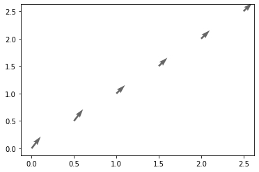
接下来是矢量图,参数具体见https://blog.csdn.net/liuchengzimozigreat/article/details/84566650

In [26]:

1
2
3
x = np.arange(0, 3, 0.5)
y = np.arange(0, 3, 0.5)
plt.quiver(x,y ,[1,1,1,1,1,1] , [2,2,1.5,1.5,1.5,1.5], angles="xy",color="#666666")#,headwidth=10,scale=40,color="#444444")

Out[26]:

1
<matplotlib.quiver.Quiver at 0x16af9f8c970>

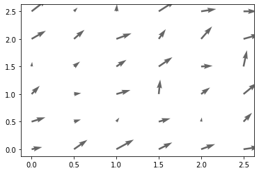
看上图其实是单点的矢量,如果要绘制矢量场则要对输入的点进行处理,也就是先meshgrid然后flatten

In [27]:

1
2
3
4
5
X, Y = np.meshgrid(x, y)
X = X.flatten()
Y = Y.flatten()
grad = np.random.rand(2,X.size)
plt.quiver(X,Y ,grad[0], grad[1], angles="xy",color="#666666")#,headwidth=10,scale=40,color="#444444")

Out[27]:

1
<matplotlib.quiver.Quiver at 0x16af9ff5f40>