import numpy as np import matplotlib.pyplot as plt from matplotlib import style import warnings from math import sqrt from collections import Counter
style.use('fivethirtyeight')
defk_nearest(dataset, test_point, k = 3): iflen(dataset) >= k: warnings.warn('K is set to a value less than total voting groups!') distances = []
for group in dataset: for feature_point in dataset[group]: euclidean_distance = sqrt((test_point[0] - feature_point[0] )**2 + (test_point[1] - feature_point[1] )**2) distances.append([euclidean_distance,group])
votes = [i[1] for i insorted(distances)[:k]] vote_result = Counter(votes).most_common(1)[0][0]
# votes contain the group character ['k', 'k', 'r'] # print(Counter(votes).most_common(1)) # You can see the Counter method also contains the #votes, so we use[0] to get['k', 2] # and [0][0] to get 'k'
# x is dimension d by 1 # th is dimension d by 1 # th0 is dimension 1 by 1 # return 1 by 1 matrix of +1, 0, -1 defpositive(x, th, th0): return np.sign(th.T@x + th0)
# Perceptron algorithm with offset. # data is dimension d by n # labels is dimension 1 by n # T is a positive integer number of steps to run # Perceptron algorithm with offset. # data is dimension d by n # labels is dimension 1 by n # T is a positive integer number of steps to run defperceptron(data, labels, params = {}, hook = None): # if T not in params, default to 100 T = params.get('T', 100) (d, n) = data.shape
theta = np.zeros((d, 1)); theta_0 = np.zeros((1, 1)) for t inrange(T): for i inrange(n): x = data[:,i:i+1] y = labels[:,i:i+1] if y * positive(x, theta, theta_0) <= 0.0: theta = theta + y * x theta_0 = theta_0 + y if hook: hook((theta, theta_0)) return theta, theta_0
Implement averaged perceptron
Regular perceptron can be somewhat sensitive to the most recent examples that it sees. Instead, averaged perceptron produces a more stable output by outputting the average value of th and th0 across all iterations.
import numpy as np # row representation defaveraged_perceptron(data, labels, params = {}, hook = None): # if T not in params, default to 100 T = params.get('T', 100)
for t inrange(T): for i inrange(n): yi = labels[:, i : i + 1] # 2-dim xi = data[i:i+1, :] # 2-dim ''' also can be written as yi = labels[0, i] # 1-dim xi = data[i] # 1-dim ''' if yi * (xi@th.T + th0) <= 0.0: th += yi * xi th0 += yi if hook: hook((th, th0)) ths += th th0s += th0
return (ths / (n * T)).T, th0s / (n * T)
Evaluating a classifier
data: a d by n array of floats (representing n data points in d dimensions)
labels: a 1 by n array of elements in (+1, -1), representing target labels
th: a d by 1 array of floats that together with
th0: a single scalar or 1 by 1 array, represents a hyperplane
1 2 3 4 5 6 7 8 9 10 11 12 13
defeval_classifier(learner, data_train, labels_train, data_test, labels_test): (d, t) = data_test.shape th = np.zeros((d, 1)); th0 = np.zeros((1, 1)) th, th0 = learner(data_train, labels_train) ans = 0 for i inrange(t): x = data_test[:,i:i+1] y = labels_test[:,i:i+1] if(np.sign(th.T@x + th0) == y): ans = ans + 1 returnfloat(ans) / k
**Evaluating a learning algorithm using a data source **
Returns a scalar number of data points that the separator correctly classified.
The eval_classifier function should accept the following parameters:
learner - a function, such as perceptron or averaged_perceptron
data_train - training data
labels_train - training labels
data_test - test data
labels_test - test labels
and returns the percentage correct on a new testing set as a float between 0. and 1.
1
2
3
4
5
6
7
8
9
defeval_learning_alg(learner, data_gen, n_train, n_test, it): ans = 0 for i inrange(it): (data_train, labels_train) = data_gen(n_train) (data_test, labels_test) = data_gen(n_test) an = eval_classifier(learner, data_train, labels_train, data_test, labels_test) ans += an return ans / it
The difference between evaluating the classifier and the learning algorithm
One classifier is just one specific result from the learning algorithm. To evaluate the learning algorithm, we can choose to average over a set of test data.
Evaluating a learning algorithm using a data source
data_gen - a data generator, call it with a desired data set size; returns a tuple (data, labels)
it - the number of iterations to average over
1
2
3
4
5
6
7
8
9
defeval_learning_alg(learner, data_gen, n_train, n_test, it): ans = 0 for i inrange(it): (data_train, labels_train) = data_gen(n_train) (data_test, labels_test) = data_gen(n_test) an = eval_classifier(learner, data_train, labels_train, data_test, labels_test) ans += an return ans / it
Evaluating a learning algorithm with a fixed dataset
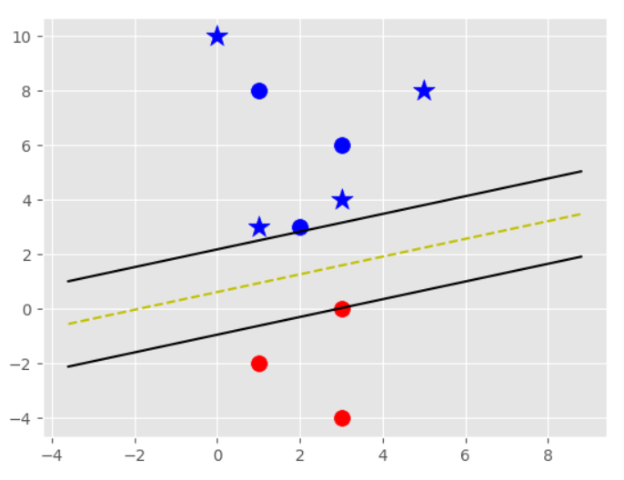
for step in step_sizes: w = np.array([latest_optimum, latest_optimum])
# we can do this because convex optimized = False whilenot optimized: for b in np.arange(-1 * (self.max_feature_value * b_range_multiple), 1 * (self.max_feature_value * b_range_multiple), step * b_multiple): for transform in transforms: w_t = w * transform found_option = True
for i in self.data: for xi in self.data[i]: yi = i ifnot yi * (np.dot(w_t, xi) + b) >= 1: found_option = False break ifnot found_option: break
if found_option: opt_dict[np.linalg.norm(w_t)] = [w_t, b]
if w[0] < 0: optimized = True print("+1 optimized\n") else: w = w - step
norms = sorted([n for n in opt_dict]) opt_choice = opt_dict[norms[0]] self.w = opt_choice[0] self.b = opt_choice[1] latest_optimum = opt_choice[0][0] * step * 2
defpredict(self, features): classification = np.sign(np.dot(self.w, np.array(features)) + self.b) if classification != 0and self.visualization: self.ax.scatter(features[0], features[1], s = 200, marker = '*', c = self.colors[classification]) return classification
defvisualize(self): [[self.ax.scatter(x[0], x[1], s=100, color=self.colors[i]) for x in data_dict[i]] for i in data_dict] # hyperplane = x.w+b # v = x.w+b # psv = 1 # nsv = -1 # dec = 0 defhyperplane(x,w,b,v): return (-w[0]*x-b+v) / w[1]
#in python, you should know that Invariant type: integer, float, long, complex, string, tuple, frozenset Variant type: list, dictionary, set, numpy array, user defined objects """" When we pass a paramter to a function, if a the variable type is variant, the inner change in the function will also cause the outter value change. """
## lambda defloss(m, n): return m - n x = 3 t = 2 f = lambda w: loss(x, t) # the same as deff(w): return loss(x, t) # This is calling another function, and x, t are arguments not parameters ans = f(x) # ans = 1 """ w is only a pseudo paramter, the reason of using lambda is to simplify coding."""
## enumerate() # iterate through an array bar = np.array([[1,2],[3, 5],[8,9]]) list(enumerate(bar)) # output: [(0, array([1, 2])), (1, array([3, 5])), (2, array([8, 9]))]
for idx,x inenumerate(bar): print(f"idx is {idx}, x is",x) """ output: idx is 0, x is [1 2] idx is 1, x is [3 5] idx is 2, x is [8 9] """
x.ndim # output: 2 x.shape # output: (4, 3) x.size # output: 12 numbers of elements x.argmax(axis = 1) # output: array([1, 2, 1, 0]) """ axis = 1 means in each row, find the max number's index """
x.reshape(1, x.size) # change x to 2d-vector form, not 1d-vector # output: array([[0.1, 0.8, 0.1, 0.3, 0.1, 0.6, 0.2, 0.5, 0.3, 0.8, 0.1, 0.6]])
x.reshape(2, 6) # output: array([[0.1, 0.8, 0.1, 0.3, 0.1, 0.6], [0.2, 0.5, 0.3, 0.8, 0.1, 0.6]]) # change x to 2 rows, 6 colunms array, in the order of row index
# matrix - 1d vector # every row minus the vector x - [0.1, 0.1, 0.1] # output: array([[0. , 0.7, 0. ], [0.2, 0. , 0.5], [0.1, 0.4, 0.2], [0.7, 0. , 0.5]]) """ The vector must have the same size as the row vector. In the softmax function, we use the traverse method to avoid the mistake. """
## numpy random # np.random.randn: array ramdom generation x = np.random.randn(2, 4) # get a 2 row, 4 column array, whose elements are correspond to normal distribution.
# np.random.choice: randomly pick numbers train_size = x_train.shape[0] batch_size = 10 batch_mask = np.random.choice(train_size, batch_size) # the same as np.random.choice(60000, 10), pick 10 numbers randomly from 0-59999, and generate an index array.
## numpy.nditer
it = np.nditer(x, flags=['multi_index'], op_flags=['readwrite']) # type: numpy.nditer

""""
np.nditer is used to iterare through an array, the parameter flags = ['multi_index'] means you can just use it.multi_index to get the index of it[0](current element) in the original array.
""""

# example
x = np.arange(6).reshape(2,3)
it = np.nditer(x, flags=['multi_index'], op_flags=['readwrite'])
while not it.finished:
    print("%d <%s>" % (it[0], it.multi_index))
    it.iternext()

# 0 <(0, 0)>
# 1 <(0, 1)>
# 2 <(0, 2)>
# 3 <(1, 0)>
# 4 <(1, 1)>
# 5 <(1, 2)>
from dataset.mnist import load_mnist
"""
    load MNIST dataset

    Parameters
    ----------
    normalize : 将图像的像素值正规化为0.0~1.0
    one_hot_label :
        one_hot_label为True的情况下,标签作为one-hot数组返回
        one-hot数组是指[0,0,1,0,0,0,0,0,0,0]这样的数组
    flatten : 是否将图像展开为一维数组

    Returns
    -------
    (训练图像, 训练标签), (测试图像, 测试标签)
"""
(x_train, t_train), (x_test, t_test) = load_mnist(normalize = True, one_hot_label = True)
""""
 x_train and t_train are array type
 x_train.shape: (60000, 784)
 t_train.shape: (60000, ) just the 1d-vector
""""
Functions
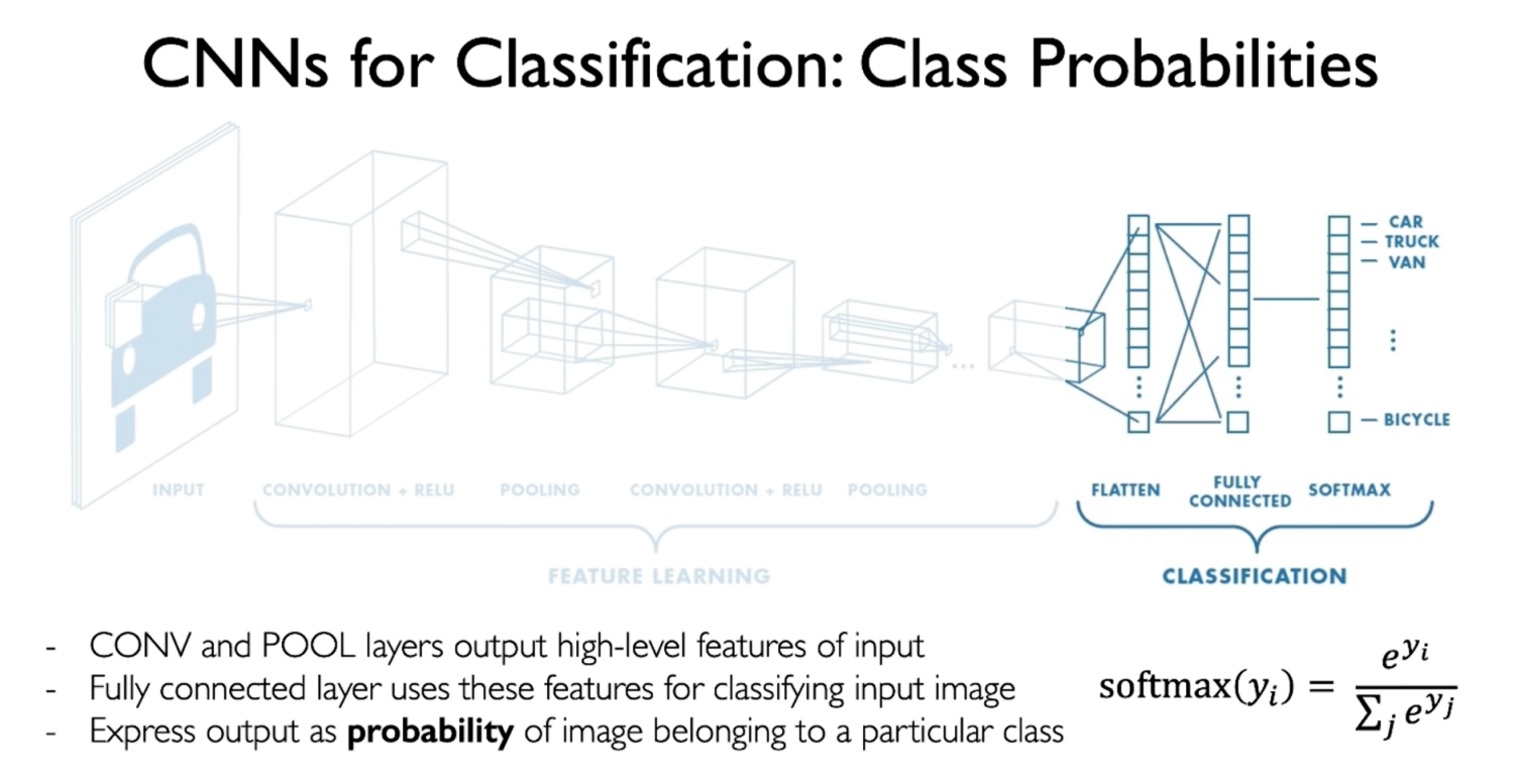
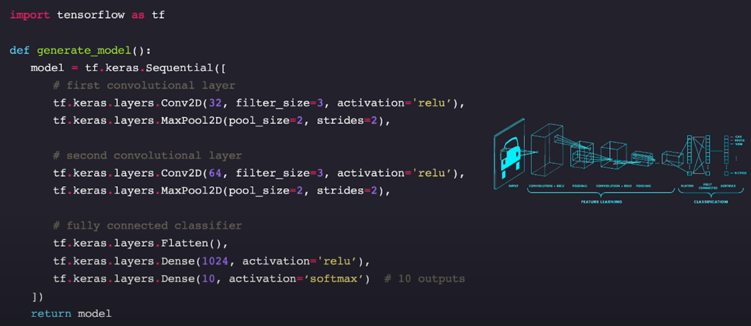
Neural network can be used in classification and regression problems, but the output needs to be changed according to the specific situation.
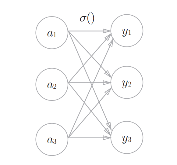
When it comes to the choice of output layer activation function, generally speaking, in the regression problem, we usually use the identity function and in the classification problem we usually use the softmax function.
Because of the property of and , we can interpret as probability. And in practice, we usually use (often chosen with the maximum number in ) to avoid overflow.
The picture above use the sigmoid function as the activation function, whereas the below one uses softmax.
# softmax defsoftmax(x): if x.ndim == 2: x = x.T x = x - np.max(x, axis = 0) y = np.exp(x) / np.sum(np.exp(x), axis = 0) return y.T x = x - np.max(x) # 1-dim case return np.exp(x) / np.sum(np.exp(x))
For the proof of this formula, you can just take 1-dimension case for example, and increase the dimension, then smoothly generalizing to the matrix form.
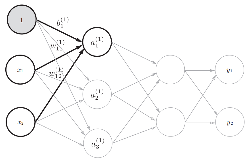
That is, to get an intuition understanding, look the following, and draw the neural connection picture to gain a feeling over the formula.
And now, just add one more dimension to see the process again:
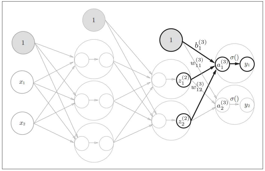
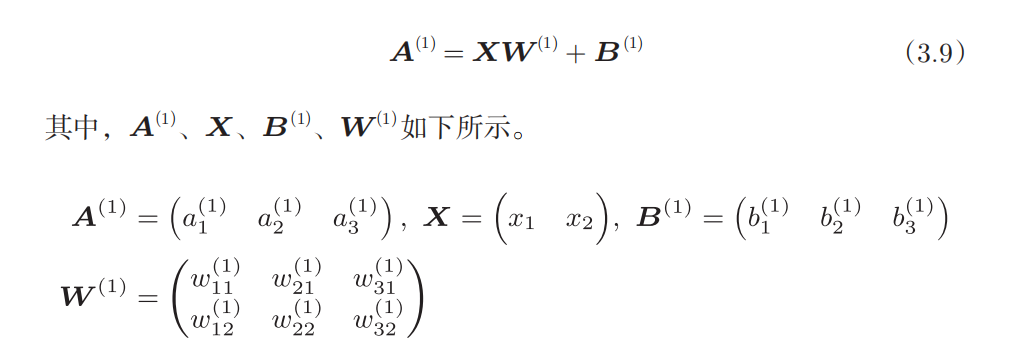
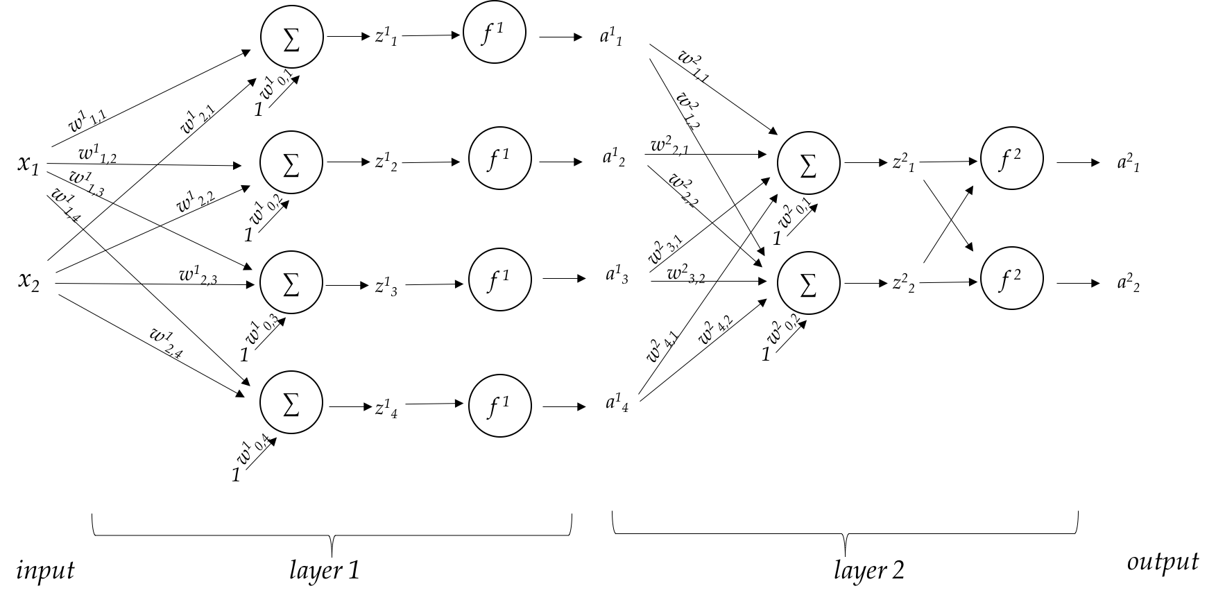
The representation of layers in the back propagation algorithm
, are the nodes in the previous representation, but now we are gonna to talk about the forward propagation and back propagation, so we need to express the transformations in each layers explicitly.
# the training part are the same import numpy as np from functions import * from gradient import * from BP_design import * from collections import OrderedDict
classTwoLayerNet: def__init__(self, input_size, hidden_size, output_size, weight_init_std = 0.01): self.params = {} # initialize # weight_init_std is the initial standard variance of weight self.params['w1'] = np.random.randn(input_size, hidden_size) * weight_init_std self.params['b1'] = np.zeros(hidden_size) self.params['w2'] = np.random.randn(hidden_size, output_size) * weight_init_std self.params['b2'] = np.zeros(output_size)
defaccuracy(self, x, t): y = self.predict(x) y = np.argmax(y, axis = 1) t = np.argmax(t, axis = 1)
accuracy = np.sum(y==t) / float(y.shape[0])
return accuracy
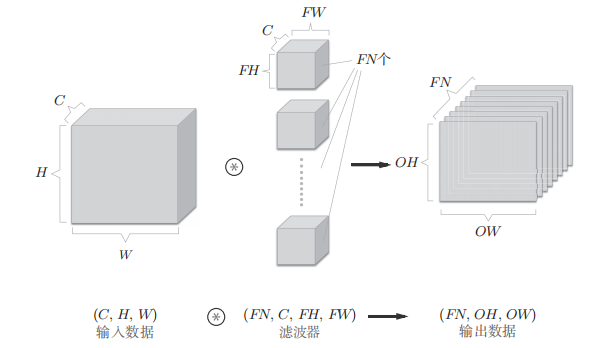
CNN
Introduction
Why CNN?
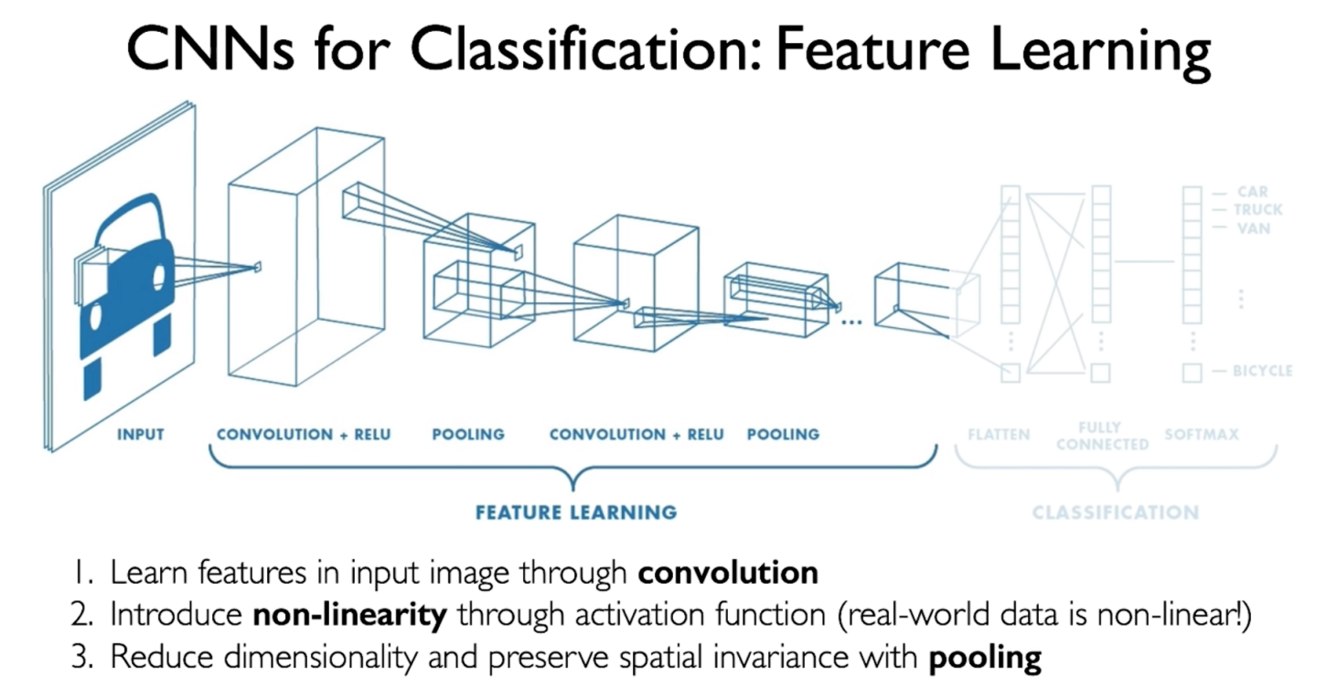
In the previous neural network, we just use the fully connected layer. However, many important spatial information are lost in the fully connected layer, such as one pixel is closer to its neighboring pixel. And also, the fully connected layer just has too many parameters, so complex.
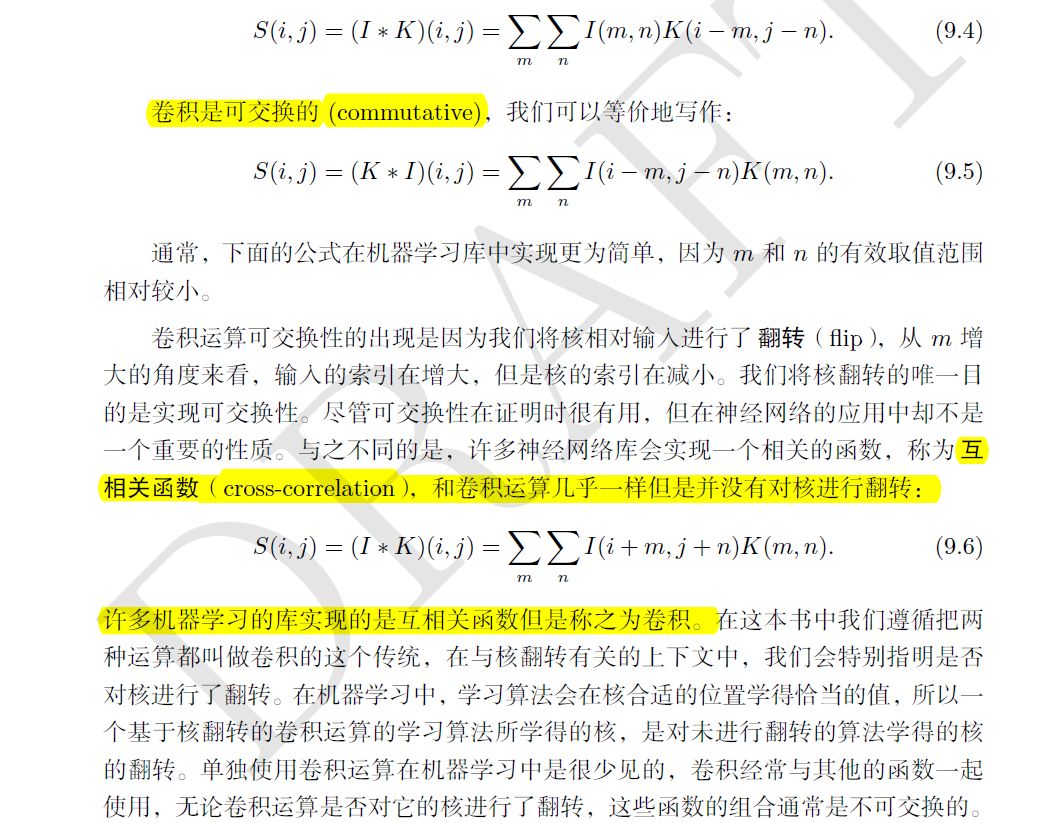
在深度学习中,卷积中的过滤器不经过反转。严格来说,这是互相关。我们本质上是执行逐元素乘法和加法。但在深度学习中,直接将其称之为卷积更加方便。这没什么问题,因为过滤器的权重是在训练阶段学习到的。如果上面例子中的反转函数 g 是正确的函数,那么经过训练后,学习得到的过滤器看起来就会像是反转后的函数 g。因此,在训练之前,没必要像在真正的卷积中那样首先反转过滤器。
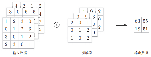
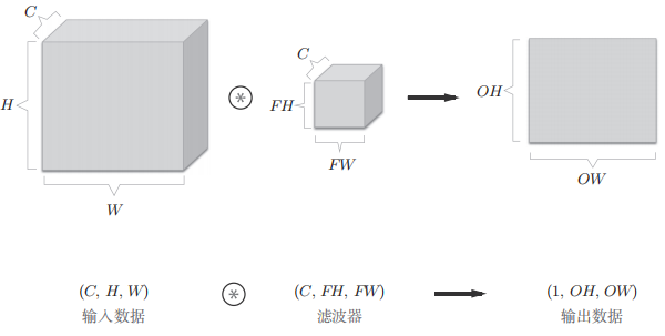
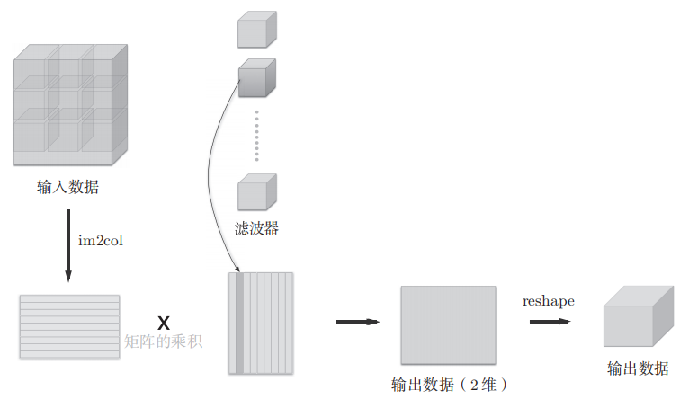
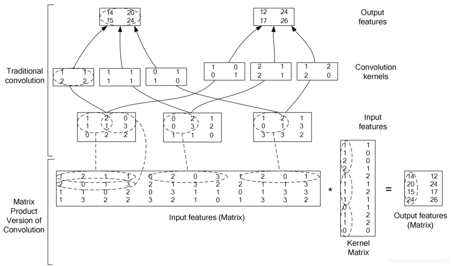
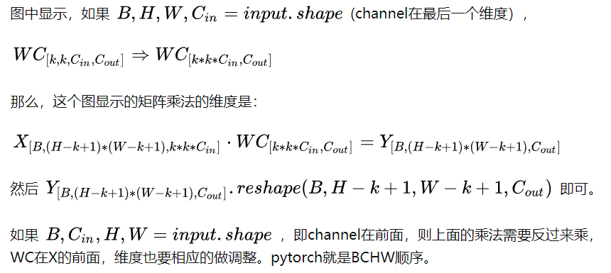
The normal convolution operation use many for loops, which behave really slowly with numpy. So, actually, we choose im2col, basically saying, it’s just reshape convolution into matrix multiplication.
In more detail, the number of cols after the im2col transform is the number of kernel traverses, the rows are the filter’s size times #channel.
import numpy as np from common.util import im2col from common.util import col2im classCovolution: def__init__(self, w, b, stride = 1, pad = 0): self.w = w self.b = b self.stride = stride self.pad = pad
defforward(self, x): N, C, H, W = x.shape out_h = int(1 + (H - self.pool_h) / self.stride) out_w = int(1 + (W - self.pool_w) / self.stride)
col = im2col(x, self.pool_h, self.pool_w, self.stride, self.pad) col = col.reshape(-1, self.pool_h * self.pool_w) # reshape can be visualized as first make the matrix 1-d with order rows to rows # and then, reshape it from the order of width, height...
out = np.max(col, axis = 1)
out = out.reshape(N, out_h, out_w, C).transpose(0, 3, 1, 2)

x
,