这次作业的任务是图像分类(classification)和图像认证(verification),值得注意的是这个分类任务是closed set problem,图像一共有7000种类别,每个图像的主体都会出现在训练集中,在测试集中该主体的图像会和测试集中的有所不同。认证的任务是open set problem,下面的图解释了这两种问题的差别。对于verification我们关注的点并不是所属哪个类别,而是这个datapoint能与其他datapoint比较的metric值。除了这点外,verification和classification的区别还在于verification是允许一对多match的,也就是一个sample和多个identity匹配,而classification只是一对一。
关于这两种任务的差别,指导书解释了一堆,有点冗余🤔
Solving Problems
分类问题利用传统的方法解决就行:
A face classifier that can extract feature vectors from face images. The face classifier consists of two main parts: the feature extractor and the classification layer.
Your model needs to be able to learn facial features (e.g., skin tone, hair color, nose size, etc.) from an image of a person’s face and represent them as a fixed-length feature vector called face embedding. In order to do this, you will explore architectures consisting of multiple convolutional layers. Stacking several convolutional layers allows for hierarchical decomposition of the input image. For example, if the first layer extracts low-level features such as lines, then the second layer (that acts on the output of the first layer) may extract combinations of low-level features, such as features that comprise multiple lines to express shapes.
为了解决这一问题,增强特征向量的鉴别能力,需要同时最大化其类内紧凑性和类间跨度,我们可以结合不同的损失函数设计最终的loss function。(Use Center loss, Sphere loss, Large-margin softmax loss, Large-margin Gaussian mixture loss etc)。Each of these losses is jointly used with cross-entropy loss to get high-quality feature vectors.
The verification task consists of the following generalized scenario:
You are given X unknown identities
You are given Y known identities
Your goal is to match X unknown identities to Y known identities.
We have given you a verification dataset, that consists of 1000 known identities, and 1000 unknown identities. The 1000 unknown identities are split into dev (200) and test (800). Your goal is to compare the unknown identities to the 1000 known identities and assign an identity to each image from the set of unknown identities.
Your will use/finetune your model trained for classification to compare images between known and unknown identities using a similarity metric and assign labels to the unknown identities.
This will judge your model’s performance in terms of the quality of embeddings/features it generates on images/faces it has never seen during training for classification.
DATA_DIR = '/content/11-785-f22-hw2p2-classification'# TODO: Path where you have downloaded the data TRAIN_DIR = os.path.join(DATA_DIR, "classification/train") VAL_DIR = os.path.join(DATA_DIR, "classification/dev") TEST_DIR = os.path.join(DATA_DIR, "classification/test")
# Transforms using torchvision - Refer https://pytorch.org/vision/stable/transforms.html
train_transforms = torchvision.transforms.Compose([ # Implementing the right transforms/augmentation methods is key to improving performance. torchvision.transforms.ToTensor(), ]) # Most torchvision transforms are done on PIL images. So you convert it into a tensor at the end with ToTensor() # But there are some transforms which are performed after ToTensor() : e.g - Normalization # Normalization Tip - Do not blindly use normalization that is not suitable for this dataset
train_dataset = torchvision.datasets.ImageFolder(TRAIN_DIR, transform = train_transforms) val_dataset = torchvision.datasets.ImageFolder(VAL_DIR, transform = val_transforms) # You should NOT have data augmentation on the validation set. Why?
# This one-liner basically generates a sorted list of full paths to each image in the test directory self.img_paths = list(map(lambda fname: os.path.join(self.data_dir, fname), sorted(os.listdir(self.data_dir))))
Now let’s consider how do we take convolutions and assemble them into a strong architecture, considering layers, channel size, stride, kernel size etc. In this part, i’ll first cover 3 aritectures:
MobileNetV2: A fast, parameter-efficient model
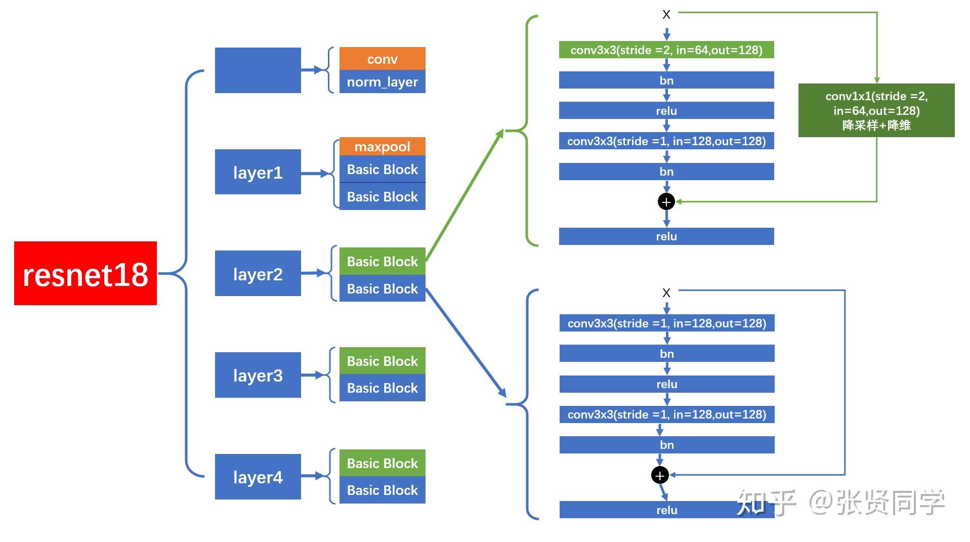
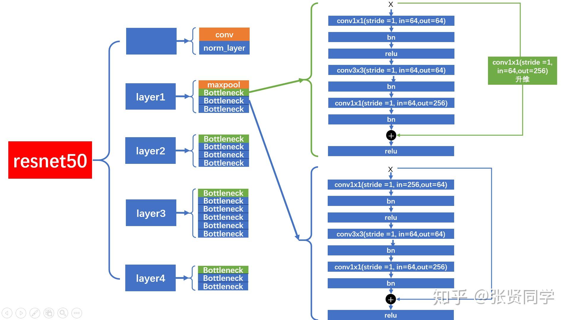
ResNet: The “go-to” for CNNs
ConvNeXt: The state of the art model
CNN architectures are divided into stages, which are divided into blocks.
Each “stage” consists of (almost) equivalent “blocks”
Each “block” consists of a few CNN layers, BN, and ReLUs
To understand an architecture, we mostly need to understand its blocks. All that changes for blocks in different stages is the base num of channels. We do need to piece these blocks together into a final model. The general flow is like this:
Stem (some linear layers like project 3 channels to 64 channels and downsample)
Stage 1
…
Stage n
Classification layer
The stem usually downsamples the input by 4x. Some stages do downsample. If they do, generally, the first convolution in the stage downsamples by 2x. When you downsample by 2x, you usually increase channel dimension by 2x. So, later stages have smaller spatial resolution, higher num of channels.
The goal of MobileNetV2 is to be parameter efficient. They do so by making extensive use of depth-wise convolutions and point-wise convolutions, which is the intuition that a normal convolution can be divided into these 2 parts but with cheaper params.
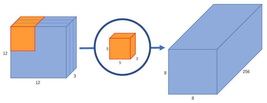
A normal convolution mixes information from both different channels and different spatial locations(pixels).
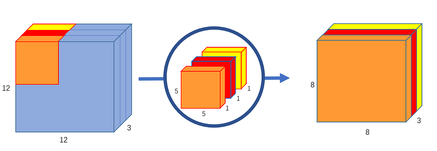
A depth-wise convolution only mixes information over spatial locations: different channels don’t interact. “Depth” means each channel.
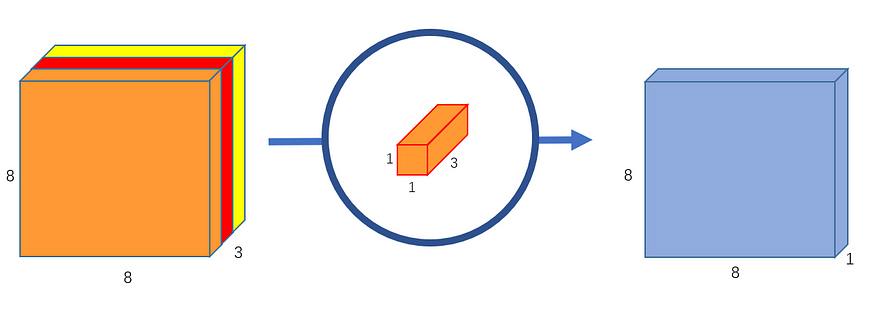
A point-wise convolution only mixes information over different channels: different spatial locations don’t interact. “point” means pixel.
MobileNetV2 Block design
First we apply a point-wise convolution to get more channels by an expansion ratio, then apply a depth-wise convolution that communicates information over different spatial locations. At last, we do a point-wise convolution but to reduce channels, which bottlenecks channels. The intuition is to distill a sparse space to a more condensed rich feature dimension.
classInvertedResidualBlock(nn.Module): """ Intuitively, layers in MobileNet can be split into "feature mixing" and "spatial mixing" layers. You can think of feature mixing as each pixel "thinking on its own" about its own featuers, and you can think of spatial mixing as pixels "talking with each other". Alternating these two builds up a CNN. In a bit more detail: - The purpose of the "feature mixing" layers is what you've already seen in hw1p2. Remember, in hw1p2, we went from some low-level audio input to semantically rich representations of phonemes. Featuring mixing is simply a linear layer (a weight matrix) that transforms simpler features into something more advanced. - The purpose of the "spatial mixing" layers is to mix features from different spatial locations. You can't figure out a face by looking at each pixel on its own, right? So we need 3x3 convolutions to mix features from neighboring pixels to build up spatially larger features. """ def__init__(self, in_channels, out_channels, stride, expand_ratio): super().__init__() # Just have to do this for all nn.Module classes
# Can only do identity residual connection if input & output are the # same channel & spatial shape. if stride == 1and in_channels == out_channels: self.do_identity = True else: self.do_identity = False # Expand Ratio is like 6, so hidden_dim >> in_channels hidden_dim = in_channels * expand_ratio
""" What is this doing? It's a 1x1 convolutional layer that drastically increases the # of channels (feature dimension). 1x1 means each pixel is thinking on its own, and increasing # of channels means the network is seeing if it can "see" more clearly in a higher dimensional space. Some patterns are just more obvious/separable in higher dimensions. Also, note that bias = False since BatchNorm2d has a bias term built-in. As you go, note the relationship between kernel_size and padding. As you covered in class, padding = kernel_size // 2 (kernel_size being odd) to make sure input & output spatial resolution is the same. """ self.feature_mixing = nn.Sequential( # TODO: Fill this in! nn.Conv2d(in_channels=in_channels, out_channels=hidden_dim, kernel_size=1, stride=1, padding=0, bias=False), nn.BatchNorm2d(hidden_dim), nn.ReLU6(inplace=True) )
""" What is this doing? Let's break it down. - kernel_size = 3 means neighboring pixels are talking with each other. This is different from feature mixing, where kernel_size = 1. - stride. Remember that we sometimes want to downsample spatially. Downsampling is done to reduce # of pixels (less computation to do), and also to increase receptive field (if a face was 32x32, and now it's 16x16, a 3x3 convolution covers more of the face, right?). It makes sense to put the downsampling in the spatial mixing portion since this layer is "in charge" of messing around spatially anyway. Note that most of the time, stride is 1. It's just the first block of every "stage" (layer \subsetof block \subsetof stage) that we have stride = 2. - groups = hidden_dim. Remember depthwise separable convolutions in class? If not, it's fine. Usually, when we go from hidden_dim channels to hidden_dim channels, they're densely connected (like a linear layer). So you can think of every pixel/grid in an input 3 x 3 x hidden_dim block being connected to every single pixel/grid in the output 3 x 3 x hidden_dim block. What groups = hidden_dim does is remove a lot of these connections. Now, each input 3 x 3 block/region is densely connected to the corresponding output 3 x 3 block/region. This happens for each of the hidden_dim input/output channel pairs independently. So we're not even mixing different channels together - we're only mixing spatial neighborhoods. Try to draw this out, or come to my (Jinhyung Park)'s OH if you want a more in-depth explanation. https://towardsdatascience.com/a-basic-introduction-to-separable-convolutions-b99ec3102728 """ self.spatial_mixing = nn.Sequential( # TODO: Fill this in! nn.Conv2d(in_channels=hidden_dim, out_channels=hidden_dim, kernel_size=3, stride=stride, padding=1, groups=hidden_dim, bias=False), nn.BatchNorm2d(hidden_dim), nn.ReLU6(inplace=True) )
""" What's this? Remember that hidden_dim is quite large - six times the in_channels. So it was nice to do the above operations in this high-dim space, where some patterns might be more clear. But we still want to bring it back down-to-earth. Intuitively, you can takeaway two reasons for doing this: - Reduces computational cost by a lot. 6x in & out channels means 36x larger weights, which is crazy. We're okay with just one of input or output of a convolutional layer being large when mixing channels, but not both. - We also want a residual connection from the input to the output. To do that without introducing another convolutional layer, we want to condense the # of channels back to be the same as the in_channels. (out_channels and in_channels are usually the same). """ self.bottleneck_channels = nn.Sequential( # TODO: Fill this in! nn.Conv2d(in_channels=hidden_dim, out_channels=out_channels, kernel_size=1, stride=1, padding=0, bias=False), nn.BatchNorm2d(out_channels) )
defforward(self, x): out = self.feature_mixing(x) out = self.spatial_mixing(out) out = self.bottleneck_channels(out)
if self.do_identity: return x + out else: return out
classMobileNetV2(nn.Module): """ The heavy lifting is already done in InvertedBottleneck. Why MobileNetV2 and not V3? V2 is the foundation for V3, which uses "neural architecture search" to find better configurations of V2. If you understand V2 well, you can totally implement V3! """ def__init__(self, num_classes= 7000): super().__init__()
self.num_classes = num_classes
""" First couple of layers are special, just do them here. This is called the "stem". Usually, methods use it to downsample or twice. """ self.stem = nn.Sequential( # TODO: Fill this in! nn.Conv2d(3, 32, 3, 2, 1, bias=False), nn.BatchNorm2d(32), nn.ReLU6(inplace=True), nn.Conv2d(32, 32, 3, 1, 1, groups=32, bias=False), nn.BatchNorm2d(32), nn.ReLU6(inplace=True), nn.Conv2d(32, 16, 1, 1, 0, bias=False), nn.BatchNorm2d(16), )
""" Since we're just repeating InvertedResidualBlocks again and again, we want to specify their parameters like this. The four numbers in each row (a stage) are shown below. - Expand ratio: We talked about this in InvertedResidualBlock - Channels: This specifies the channel size before expansion - # blocks: Each stage has many blocks, how many? - Stride of first block: For some stages, we want to downsample. In a downsampling stage, we set the first block in that stage to have stride = 2, and the rest just have stride = 1. Again, note that almost every stage here is downsampling! By the time we get to the last stage, what is the image resolution? Can it still be called an image for our dataset? Think about this, and make changes as you want. """ self.stage_cfgs = [ # expand_ratio, channels, # blocks, stride of first block [6, 24, 2, 2], [6, 32, 3, 2], [6, 64, 4, 2], [6, 96, 3, 1], [6, 160, 3, 2], [6, 320, 1, 1], ]
# Remember that our stem left us off at 16 channels. We're going to # keep updating this in_channels variable as we go in_channels = 16
# Let's make the layers layers = [] for curr_stage in self.stage_cfgs: expand_ratio, num_channels, num_blocks, stride = curr_stage for block_idx inrange(num_blocks): out_channels = num_channels layers.append(InvertedResidualBlock( in_channels=in_channels, out_channels=out_channels, # only have non-trivial stride if first block stride=stride if block_idx == 0else1, expand_ratio=expand_ratio )) # In channels of the next block is the out_channels of the current one in_channels = out_channels self.layers = nn.Sequential(*layers) # Done, save them to the class
# Some final feature mixing self.final_block = nn.Sequential( nn.Conv2d(in_channels, 1280, kernel_size=1, padding=0, stride=1, bias=False), nn.BatchNorm2d(1280), nn.ReLU6() )
# Now, we need to build the final classification layer. self.avgpool = nn.AdaptiveAvgPool2d((1, 1)) self.classifier = nn.Linear(1280, self.num_classes)
self._initialize_weights()
def_initialize_weights(self): """ Usually, I like to use default pytorch initialization for stuff, but MobileNetV2 made a point of putting in some custom ones, so let's just use them. """ for m in self.modules(): ifisinstance(m, nn.Conv2d): n = m.kernel_size[0] * m.kernel_size[1] * m.out_channels m.weight.data.normal_(0, math.sqrt(2. / n)) if m.bias isnotNone: m.bias.data.zero_() elifisinstance(m, nn.BatchNorm2d): m.weight.data.fill_(1) m.bias.data.zero_() elifisinstance(m, nn.Linear): m.weight.data.normal_(0, 0.01) m.bias.data.zero_()
defforward(self, x, return_feats=False): out = self.stem(x) out = self.layers(out) out = self.final_block(out)
#the shortcut output dimension is not the same with residual function #use 1*1 convolution to match the dimension if stride != 1or in_channels != BasicBlock.expansion * out_channels: self.shortcut = nn.Sequential( nn.Conv2d(in_channels, out_channels * BasicBlock.expansion, kernel_size=1, stride=stride, bias=False), nn.BatchNorm2d(out_channels * BasicBlock.expansion) )
def_make_stage(self, block, out_channels, num_blocks, stride): """make resnet layers(by layer i didnt mean this 'layer' was the same as a neuron netowork layer, ex. conv layer), one layer may contain more than one residual block Args: block: block type, basic block or bottle neck block out_channels: output depth channel number of this layer num_blocks: how many blocks per layer stride: the stride of the first block of this layer Return: return a resnet layer """
# we have num_block blocks per layer, the first block # could be 1 or 2, other blocks would always be 1 strides = [stride] + [1] * (num_blocks - 1) layers = [] for stride in strides: layers.append(block(self.in_channels, out_channels, stride)) self.in_channels = out_channels * block.expansion
SOTA architecture, its intuitions are very similar to MobileNetV2.
The differences:
The depth-wise convolution in ConvNeXt is larger kernel size(7x7).
The order of spatial mixing & feature mixing are flipped. In ConvNeXt, depth-wise convolution operates on lower num of channels. In MobileNetV2, operates on higher num of channels.
Channel Expansion Ratio in ConvNeXt is 4, MobileNetV2 is 6
You will find that even when using a larger/more advanced model, that modal might have same/worse performance. That’s because the larger model is severely overfitting.


(也就是不变)
(也就是不变)


.png)