HW1P1

  In this HW, i’m gonna to complete the basic MLP (aka the simplest NN) by designing my own mytorch library which can be reused in the subsequent HW

  Here is the layout of this note (blog):

1. Brief Introduction
2. Python Implementation
3. Torch Pipeline

Introduction

Representation

  MLPs are universal function approximators , they can model any Boolean function, classification function, or regression. Now, I will explain this powerful representation ability in an intuitive way.

  First, MLPs can be viewed as universal Boolean functions, because perceptrons can modelAND , OR, NOT gate. Any truth table can be expressed in one-hidden-layer MLP, if we just get every item from the table and compose an expression, it costs neurons.

  But what if using more layers instead of just one-hidden-layer, by increasing the depth of the network, we are able to use less perceptrons, because it captures the relations between neurons.

  The decision boundary captured by the boolean network can be any convex region, and can be composed together by adding one more layer to get a bigger maybe non-convex region. In this way, we can get any region we want in theory.

 But can one-hidden-layer MLP model all the decision boundary, in another word, is one-hidden-layer MLP a universal classifier?

  The answer is YES, the intuition behind this is as follows. Consider now we want to model , when we push to infinite, we will get a circle region in 2d, and a cylinder in 3d.

  So in theory, we can achieve this:

  But this is true only when N is infinite, this actually won’t work in practice. However, deeper networks can require far fewer neurons– 12 vs. ~infinite hidden neurons in this example. And in many cases, increase the depth can help a lot, a special case for this is the sum-product problem, also can be viewed as kind of DP idea.

  How can MLP model any function? The intuition is as behind:

  The network is actually a universal map from the entire domain of input values to the entire range of the output activation

  Next i will cover the trade-off between width, depth and sufficiency of architecture. Not all architectures can represent any function. If your layers width is narrow, and without proper activation function, the network may be not sufficient to represent some functions. However, narrow layers can still pass information to subsequent layers if the activation function is sufficiently graded. But will require greater depth, to permit later layers to capture patterns.

  In a short summary, deeper MLPs can achieve the same precision with far fewer neurons, but must still have sufficient capacity:

• The activations must pass information through

• Each layer must still be sufficiently wide to convey all relevant information to subsequent layers.

  There are some supplement material analyzing the “capacity” of a network using VC dimension. I don’t want to cover them all here. :)

  Then here let me introduce a variant network called RBF network. If you know Kernel SVM before, you must be familiar with the word RBF. So a RBF network is like this:

  The difference between RBF network and BP network lies on the way they combine weights and inputs, see more here link.

  RBF network is the best approximation to continuous funcitons:

  See more material on RBFNN and SVM, RBFNN and GMM

Learning

  We know that MLP can be constructed to represent any function, but there is a huge gap between “can” and “how to”. One naive approach is to handcraft a network to satisfy it, but only for the simplest case. More generally, given the function to model, we want to derive the parameters of the network to model it, through computation. We learn networks (The network must have sufficient capacity to model the function) by “fitting” them to training instances drawn from a target function. Estimate parameters to minimize the error between the target function and the network function .

  But is unknow, we only get the sampled input-output pairs for a number of samples of input , , where . We must learn the entire function from these few “training” samples.

  For classification problem, there’s an old method called perceptorn algorithm. So i’ll only cover the main idea here, which is the update rule. Everytime we mis-classified a data point, we adjust our vector to fit this point. The detailed proof can be found in mit 6.036.

  So can we apply the perceptron algorithm idea to the training process of MLP using the threshold function? The answer is NO. Even using the perfect architecture, it will still cost exponential time because we are using threshold function, so nobody tells us how far is it to the right answer, we have to try out every possible combinations.

  Suppose we get every perceptron right except for the yellow cricle one, we need to train it to get the line as follows:

  The individual classifier actually requires the kind of labelling shown below which is not given. So we need to try out every possible way of relabeling the blue dots such that we can learn a line that keeps all the red dots on one side

  So how to get rid of this limitation? In fact, it costs people more than a decade to give the solution XD. The problem is binary error metric is not useful, there is no indication of which direction to change the weights to reduce error, so we have to try out every possibility.

  The solution is to change our way of computing the mismatch such that modifying the classifier slightly lets us know if we are going the right way or no.

• This requires changing both, our activation functions, and the manner in which we evaluate the mismatch between the classifier output and the target output
• Our mismatch function will now not actually count errors, but a proxy for it

  So we need our mismatch function to be differentiable. Small changes in weight can result in non-negligible changes in output. This enables us to estimate the parameters using gradient descent techniques.

  Come back to the problem of learning, we use divergence ( actually a Functional, take function as input, output a number ) to measure the mismatch, which is an abstract compared with the error defined before. Because when we are talking about “Error”, this is often referred to the data-point-wise terminology, and we use “Total Error” to measure the overall dismatch. But when we step into the probability distribution world, this is not sufficient enough, so we proposed the concept of divergence, just an abstract of the “Error” we talked before.

  Divergence is a functional, because we want to measure the difference between functions given the input. We don’t really care about the input here, because we just use all the input values to calculate the divergence. We are more concerned about the relation between output of the divergence and the weights( which determines how our changes).

 More generally, assuming is a random variable, we don’t need to consider the range we never cover, so we introduce the expectation to get the best :

  We used the concept “Risk” associated with hypothesis , which is defined as follows:

  In practice, we can only get few sampled data, so we need to define “Empirical risk”:

 Its really a measure of error, but using standard terminology, we will call it a “Loss” . The empirical risk is only an empirical approximation to the true risk which is our actual minimization objective. For a given training set the loss is only a function of W.

  Breif summary: We learn networks by “fitting” them to training instances drawn from a target function. Learning networks of threshold-activation perceptrons requires solving a hard combinatorial-optimization problem.Because we cannot compute the influence of small changes to the parameters on the overall error. Instead we use continuous activation functions with non-zero derivatives to enables us to estimate network parameters. This makes the output of the network differentiable w.r.t every parameter in the network– The logistic activation perceptron actually computes the a posteriori probability of the output given the input. We define differentiable divergence between the output of the network and the desired output for the training instances. And a total error, which is the average divergence over all training instances. We optimize network parameters to minimize this error–Empirical risk minimization. This is an instance of function minimization

Backpropagation

  In the previous part, we have talked about Empirical risk minimization, which is a kind of function minimization. So it’s natural to use gradient decent to optimize the objective function. The big picture of training a network(no loops, no residual connections) is described as the following.

 As you see, the first step of gradient decent is to calculate the gradient of the loss value with respect to the parameters. In this section, I will introduce backpropagatoin, which is a really efficient way to calculate gradient on the network.

  Our goal is to calculate on the network, the naive approach is to just calculate one by one without using the properties of a network, which costs unacceptable computation. A more reasonable way is to take the idea of chain rule and dynamic programming into consideration, which is backpropagation.

 Here are the assumptions (All of these conditions are frequently not applicable):

1. The computation of the output of one neuron does not directly affect computation of other neurons in the same (or previous) layers
2. Inputs to neurons only combine through weighted addition
3. Activations are actually differentiable

  So now let’s work on the math part. Actually, we just need to figure out one layer’s computation, since the other layers’ calculations are actually similar. I will choose to start from the end of the network.

  Start from the grey box (loss function calculation):

 Then we walk through the activation function:

 We get the desired gradient on layer N, Yeah~. But it’s not the time for cheering up, we have to move forward because we just computed one layer gradients, the backpropagation is still continuing. So we also have to calculate the derivative with respect to .

  Afer iteratively calculating gradients like this till the last layer, backpropagation is finished. So let me take a brief summary bellow:

 In our assumptions, the activation function is scale-wise and all the fucntions are differentiable, but we don’t get the two conditions in many cases. So for vector activation function, we need to do one more summation, and instead of directly using the gradient, we can choose subgradients sometimes.

  The matrix form is as the following, and i think the only equation needed to be clarify is the term , note that the dim of the derivative of a scaler with respect to a vector or matrix is the same as its transpose dim. And the dim of this expression looks resonable right?

 Now i’m gonna show you the math in detail. Our convention is to multiply gradient on the left, so to calculate the derivative , we need to transpose the expression to get . By applying the chain rule, we can get:

  Adding transpose, we get:

做了CMU的实验以后发现指导书写的和课堂上讲的不一样XD，课上讲的是分子布局，实验是分母布局，所以下面会把矩阵求导讲的全一点，争取切割这一节。

向量（或者标量）对向量的导数很简单，Jacobian就够了，这个我在HW0讲的比较细了，主要还是讨论一下矩阵对矩阵求导。接下来我讲的内容只是针对深度学习里的矩阵求导，因为可能不同领域对这块定义不一样，我也不太懂hh。

引用b乎大佬的回答，算是对矩阵求导做了一个定义：

来举个栗子吧，，
其中

那么

其实相当于扩展了Jacobian的定义，即中每一个元素，对于中每一个元素进行求导。转化成标量的形式就好理解了吧~至于把以上16个标量求导写成的矩阵也好还是16维的向量也好，大多是为了形式（理论）上的美观，或是方便对求导结果的后续使用，亦或是方便编程实现，按需自取，其本质不变。

对于上面的例子，数学上的答案应该是，其中 是kronecker积，kronecker product的定义可以看这里 here ，具体为啥是这结果可以看矩阵求导术。在机器学习里，我们的答案只是（分子布局），因为没有必要考虑其余的冗余项。

下面来介绍分子布局和分母布局的区别，贴一段CMU的解释：

A handy way to distinguish numerator vs denominator layout is to remember that the layout type corresponds the number of rows in the output matrix. In a numerator layout, the output matrix has number of rows equal to the size of the numerator, while in a denominator layout, the output matrix has number of rows equal to the size of the denominator.

对于ML和DL，处理的是优化问题，我们一般取分母布局，贴一段Stanford的解释：：

Jacobean formulation is great for applying the chain rule: you just have to multiply the Jacobians. However, when doing SGD it’s more convenient to follow the convention “the shape of the gradient equals the shape of the parameter” (as we did when computing ). That way subtracting the gradient times the learning rate from the parameters is easy. We expect answers to homework questions to follow this convention. Therefore if you compute the gradient of a column vector using Jacobian formulation, you should take the transpose when reporting your final answer so the gradient is a column vector. Another option is to always follow the convention. In this case the identities may not work, but you can still figure out the answer by making sure the dimensions of your derivatives match up. Up to you which of these options you choose!

使用分母布局还会导致链式法则的方向问题，这个也很容易理解，分子布局在结果上和分母布局是转置，对应他们的链式方向也会相反：

Chain rule in matrix calculus is similar to the usual chain rule in 1-dimension, with the exception that in the denominator layout, the order in which we multiply the derivatives is reversed, i.e. successive derivatives are written to the left (this is opposite for the numerator layout). For instance, in 1-dimension, if we have , then ${dy \over dx} = {dg \over dh}{dh \over dk}{dk \over dx} $ . However, if we are considering the denominator layout vector derivatives, then it is instead Technically, order doesn’t matter in 1-D cases, but it matters for vectors since the shapes have to align

对于神经网络，因为本质上我们还是在处理一个多元函数的优化，最后得到的是一个scalar，矩阵的形式只是组织结果的一种方式，我们把不同的batch组合到一个矩阵中，由于对loss的计算使用的是sum操作，也就是不同batch分别计算loss然后加起来， 也就是说，神经网络里面的所有weight和输入其实是可以写到一个scalar的式子中的，我们只是用矩阵求导这种方式来组织对应的导数，写成和原参数一样的shape是为了方便更新参数，这也让我们默认选择了分母布局，同时因为这只是我们的组织形式，也就失去了一些梯度导数原本的性质，比如梯度和的乘积表示对目标函数的增益。

下面举个例子（沿用b乎大佬的例子）：

假设batch size为3，列向量表示样本，可以得到

对于其中的某个sample而言，不妨取第一列：

从而

这里的求和其实就是关键所在，我们是利用batch计算出的梯度和进行更新，为了使求出的导数直接可以更新参数，我们把对的导数组织为下面的形式，而这在形式上是等价于分母布局的，因为shape要去align：

下面求 :

对分母布局，考虑求导方向性+加个转置就行了。lab中的例子是：

对于作业上的求导结果是这样的，可能唯一还需要想想的就是第一个式子，按道理不应该第一项的应该加上转置么（因为是分母布局），实际上因为链式法则也是有方向性，分母布局都是把新项导数的转置乘在左侧的（详细的解释看上面的例子和下面的总结），我们需要先把转置，得到的形式，再去对求导，然后再把答案转置过来就能得到结果了。

For any linear equation of the kind , the derivative of with respect to is . The derivative of with respect to is . Also the derivative with respect to a transpose is the transpose of the derivative, so the derivative of with respect to is but the derivative of with respect to is .

总结下就是:

这结论在 是一个向量的时候也成立, 即:

如果要求导的自变量在左边, 线性变换在右边, 也有类似稍有不同的结论如下, 证明方法是类似的, 这里直接给出结论:

一个记忆的小技巧就是在Jacobian分子布局下对求导就是，对分母布局就是相反着来即可。

最后还是提一嘴，别犯迷糊了，算出来的梯度是用来更新原参数的，也就是相当于的感觉，因为是多元函数，所以最后对目标函数的增益应该是，之前太久没看这部分晕了一次。

参考资料：https://github.com/FelixFu520/README/blob/main/train/optim/matrix_bp.md

Matrix Calculation

上面总结了神经网络中的矩阵求导的由来，算是ML中的矩阵求导的特例，下面我会简略介绍一般意义上的标量对矩阵求导方法，主要参考矩阵求导术link，他这篇文章默认的就是分母布局.

全微分可以写成导数矩阵和全微分矩阵的内积，这就提供了一种以矩阵形式来看待求导过程的视角，也就是整体性，基于此还需要定义一些有用的矩阵微分法则。

观察一下可以断言，若标量函数f是矩阵X经加减乘法、逆、行列式、逐元素函数等运算构成，则使用相应的运算法则对f求微分，再使用迹技巧给套上迹并将其它项交换至左侧，对照导数与微分的联系，即能得到导数。

如果和能直接联系起来，就直接全微分，如果中间夹了个其他变量，不能简单套个链式法则，一定要按照矩阵全微分的定义来****，然后去求。

具体b乎上给了很多常见的例子，受用良多。

Optimization

用英文写好累哇，开摆了，以后中英混着写，可能只有自己看得懂吧🤣，hh还是要保证通俗易懂

Material

参考资料：

http://deeplearning.cs.cmu.edu/F22/document/slides/lec6.optimization.pdf

http://deeplearning.cs.cmu.edu/F22/document/slides/lec7.stochastic_gradient.pdf

文章框架按照下面两个blog叙述，具体的细节和组织方式会丰富很多：

https://blog.paperspace.com/intro-to-optimization-in-deep-learning-gradient-descent/

https://blog.paperspace.com/intro-to-optimization-momentum-rmsprop-adam/

Basic conceptions

首先还是来介绍一些基础的概念和idea，会从最简单的梯度、海塞矩阵、泰勒展开谈起，我会分享我的一些思考方式。然后会介绍二次优化的方法，再过渡到神经网络的优化方法。

梯度能反映增长最快的方向，这个可以从hyperplane的角度去理解，可以参考b乎的这个回答 here。二阶导除了可以理解为导数的增长率，还可以从原函数局部均值的角度理解，也就是Laplace 算子的角度，可以参考这个视频 here。多元函数的泰勒展开可以写作矩阵乘法的形式其实也是从scale推的，二阶的展开推导可以看这里 here。

接下来就是和凸优化有关的理论了，对最简单的二次优化，其实牛顿法就可以给出每次更新的最优方向和步长，其实也就是泰勒二阶展开后，计算得到的最优值，一维scale的情况时，这个最优的学习率其实就是二阶导的倒数，而对于多元变量，就变成了海塞矩阵的逆了。

有关Lipschitz平滑、强对偶的理论直观上的感受可以看这里here，和梯度下降收敛性证明的有关理论可以看这个 here，还有这里 here (加拿大的学校的教学资料是真好啊)，详细的我就不介绍了。大概就是说强突的收敛的会更快，如果只是Lipschitz平滑也能收敛。

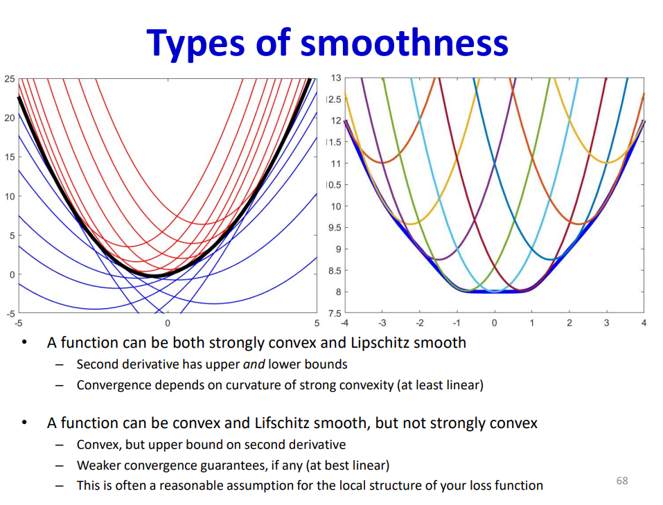
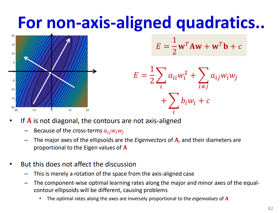
现在来讲讲海塞矩阵特征值和收敛的关系，我们知道通过二阶展开可以得到局部的近似，这个近似在局部最值附近的等值线体现为一个椭圆，而这个椭圆的长短轴就是和海塞矩阵的特征值成比例，原因这样的，通过泰勒展开我们可以把函数近似写为二次型的表达式，对应的等值线就是二次曲线这种，长短轴和特征值的关系就很明显了，通过SVD的几何意义也很容易得到。如果海塞矩阵的条件数很大，也就是椭圆的长短轴相差很大，说明这个损失函数平面是病态的，就比较难收敛。

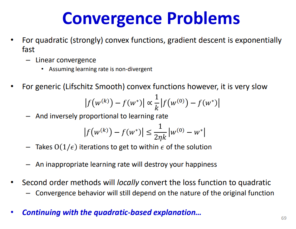
但是海塞矩阵的逆计算代价大概是的，放到神经网络里面肯定是嫩算算不出来的，也就是说对参数的每个分量确定最优的学习率是很难的，我们考虑两种不同的做法，第一种还是采取每个分量独立的学习率，但是使用启发式的思路而不是嫩算（Rprop算法），第二种就是所有分量一个学习率，就是常见的学习率直接乘梯度向量，但是这样的话收敛性就不一定能保证了，以二次优化为例，如果学习率大于任一分量最优学习率的二倍，就会发散，也由此提出了学习率衰减和收敛的理论，Robbins-Munroe conditions算是最经典的收敛条件，也就是SGD对于满足凸性和平滑的模型，只要学习率满足下面的条件就会收敛

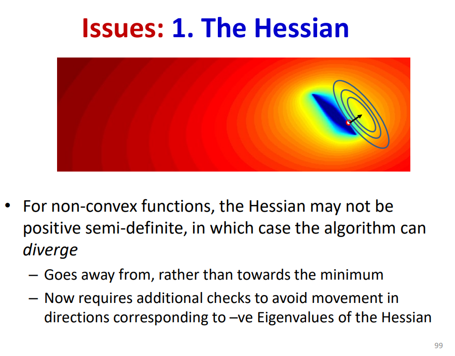
此外在梯度下降的过程中还存在主要的两个问题需要解决，针对这两个问题提出的各种解决方法就是这节的重点学习内容了。第一个问题是达不到全局最值，会收敛到局部最优点，第二个问题是对于病态的损失函数平面很可能会出现震荡的现象，导致收敛慢效果很差。

SGD and Batch

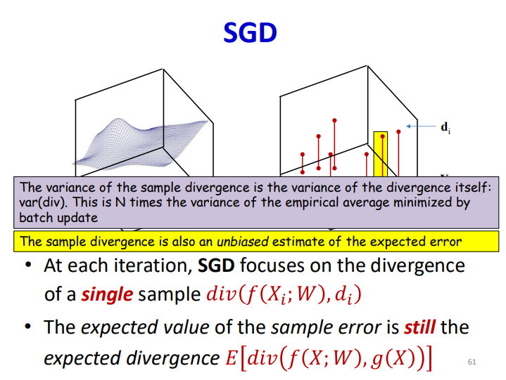
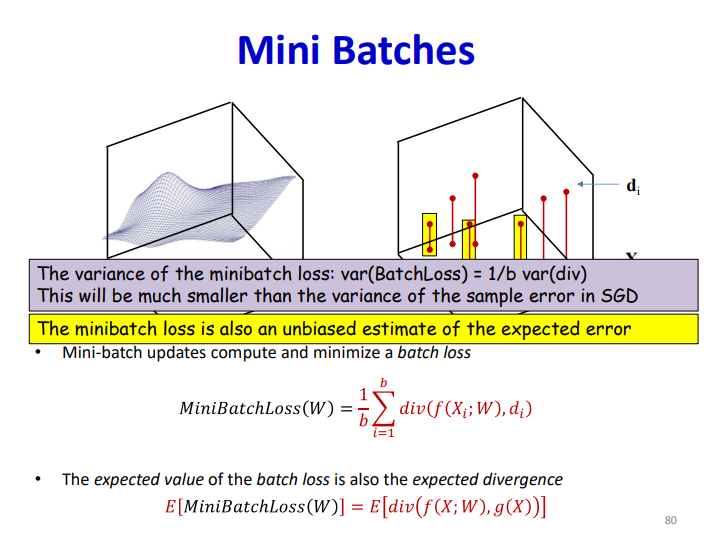
直接用全样本去计算loss function会有至少两个问题，第一个是cycle的表现，第二个是不能避免局部最值。针对这个问题，可以利用随机采样计算梯度，最简单的策略就是随机取一个样本，这是SGD的思路，但是这样会使收敛过程的方差变得很大，而且损失函数也不会变得足够小。

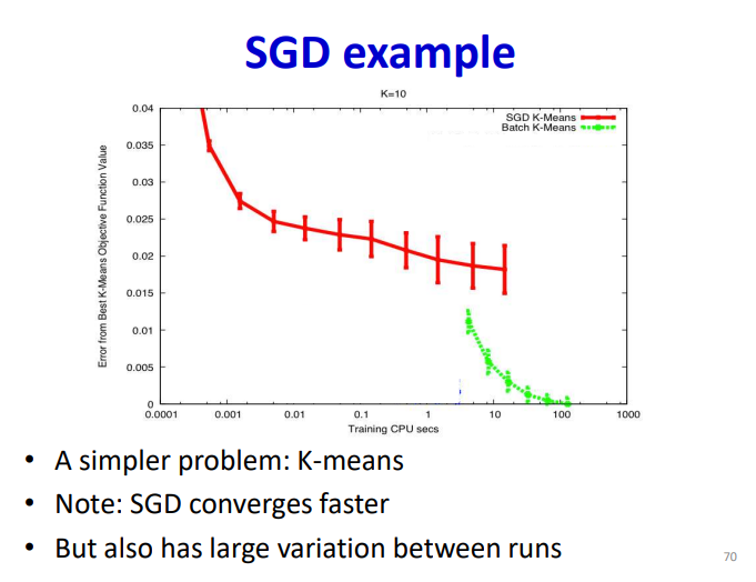
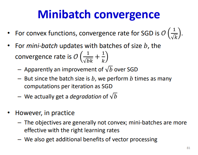
针对这个问题也是提出了mini-batch去解决，同样作为无偏估计，但是其方差缩小为原本的倍，收敛的效果也是得到了提升：

Learning Rate and Grad direction

针对病态的震荡情况，因为我们只能利用一阶导的信息，如果可以利用二阶导其实可以获得曲率等信息进行避免，但是由于计算量我们还是想一些启发式的方法去解决，未来的改进方向肯定就是何如兼顾二阶信息又减少运算量。

这部分说实话资料都很全了，值得提一嘴的是基于学习率改进的算法，AdaGrad 和 RMS Prop的关系，RMS Prop通过移动平均解决了Adagrad中平方和累加过大缺乏正则化的问题。

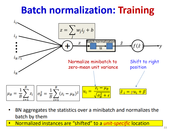
Normalization

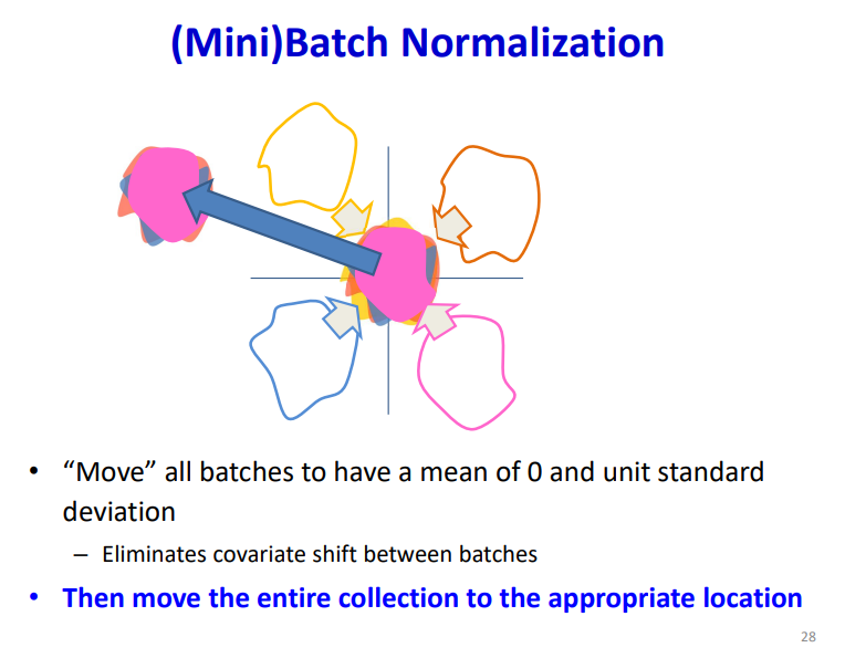
值得注意的是，使用batch-norm的话 ，线性层就不需要额外的bias项了，会被归一化掉，算是个Arbitrary的选择，可加可不加。

Python Implementation

这部分直接看我仓库吧，就不放到这里写了：code

Torch Pipeline

 Colloquially,training a model can be described like this:

1. We get data-pairs of questions and answers.

2. For a pair (x, y), we run x through the model to get the model’s answer y.

3. Then, a “teacher” gives the model a grade depending on “how wrong” y is compared to the true answer y.

4. Then based on the grade,we figure out who’s fault the error is.

5. Then, we fix the faults so the model can do better next time.

 To train a model using Pytorch, in general, there are 5 main parts:

1. Data
2. Model
3. Loss Function
4. Backpropagation
5. Optimizer

Data

 When training a model, data is generally a long list of (x, y) pairs, where you want the model to see x and predict y.

 Pytorch has two classes you will need to use to deal with data:

• torch.utils.data.Dataset
• torch.utils.data.Dataloader

 Dataset class is used to preprocess data and load single pairs (x, y)

 Dataloader class uses your Dataset class to get single pairs and group them into batches

 When defining a Dataset, there are three class methods that you need to implement 3 methods: __init__, __len__, __getitem__.

 Use __init__ to load the data to the class so it can be accessed later, Pytorch will use __len__ to know how many (x, y) pairs (training samples) are in your dataset. After using __len__ to figure out how many samples there are, Pytorch will use __getitem__ to ask for() a certain sample. So __getitem__(i) should return the “i-th” sample, with order chosen by you. You should use getitem to do some final processing on the data before it’s sent out. Since __getitem__ will be called maybe millions of times, so make sure you do as little work in here as possible for fast code. Try to keep heavy preprocessing in __init__, which is only called once

 Here is a simple Dataset example:

class MyDataset(data.Dataset):
    def __init__(self, X, Y):
        self.X = X
        self.Y = Y
      
    def __len__(self.Y):
        return len(self.Y)
    
    def __getitem(self, index):
        X = self.X[index].float().reshape(-1) #flatten the input
        Y = self.Y[index].long()
        return X, Y

 Here is a simple Dataloader example:

# Training
train_dataset = MyDataset(train.train_data, train.train_labels)

train_loader_args = dict(shuffle = True, batch_size = 256, num_workers = num_workers, pin_memory = True)\
if cuda else dict(shuffle = True, batch_size = 64)

train_loader = data.DataLoader(train_dataset, **train_loader_args)

Model

 This section will be in two parts:

• How to generate the model you’ll use

• How to run the data sample through the model.

 One key point in neural network is modularity, this means when coding a network, we can break down the structure into small parts and take it step by step.

 Now, let’s get into coding a model in Pytorch. Networks in Pytorch are (generally) classes that are based off of the nn.Module class. Similar to the Dataset class, Pytorch wants you to implement the __init__ and forward methods.

• __init__: this is where you define the actual model itself (along with other

stuff you might need)

• Forward: given an input x, you run it through the model defined in __init__

class Our_Model(nn.Module):
	def __init__(self):
        super().__init__()
        
        self.layer1 = nn.Linear(3, 4)
        self.layer2 = nn.Linear(4, 4)
        self.layer3 = nn,Linear(4, 1)
      
    def forward(self, x):
        out = self.layer1(x)
        out = self.layer2(out)
        out = self.layer3(out)
      
    	return out

 However, it can get annoying to type each of the layers twice – once in __init__ and once in forward. Since on the right, we take the output of each layer and directly put it into the next, we can use the nn.Sequential module.

class Our_Model(nn.Module):
    def __init__(self):
        layers = {
            nn.Linear(3, 4),
            nn.Linear(4, 4),
            nn.Linear(4, 1)
        }
        self.layers = nn.Sequential(*layers) # * operator opens up the lsit and directly puts them in as arguments of nn.Sequential
        
	def forward(self, x):
        return self.layers(out)

 As a beginner to Pytorch, you should definitely have link open. The documentation is very thorough. Also, for optimizers: link.

 Now that we have our model generated, how do we use it? First, we want to put the model on GPU. Note that for nn.Module classes, .to(device) is in-place. However, for tensors, you must do x = x.to(device)

device = torch.device("cuda" if cuda else "cpu")
model.to(device)

 Also, models have .train() and .eval() methods. Before training, you should run model.train() to tell the model to save gradients. When validating or testing, run model.eval() to tell the model it doesn’t need to save gradients (save memory and time). A common mistake is to forget to toggle back to .train(), then your model doesn’t learn anything.

 So far, we can build:

# Dataset Stuff
train_dataset = MyDataset(train.train_data, train.train_labels)

train_loader_args = dict(shuffle = True, batch_size = 256, num_workers = num_workers, pin_memory = True)\
if cuda else dict(shuffle = True, batch_size = 64)

train_loader = data.DataLoader(train_dataset, **train_loader_args)

# Model Stuff
model = nn.Sequential(nn.Linear(3,4 ), nn.Linear(4, 4), nn.Linear(4, 1))
device = torch.device["cuda" if cuda else "cpu"]
model.to(device)

# Optimization Stuff
NUM_EPOCHS = 100
# ----------------- #
# |	Not	cover yet | # initialize the criterion
# ----------------- #

# Training
for epoch in range(NUM_EPOCHS):
    model.train()
    
    for(x, y) in train_loaders:
        # ----------------- #
		# |	Not	cover yet | # optimizer initialize
		# ----------------- #
        x.to(device)
        y.to(device)
        
        output = model(x)
        # ----------------- #
		# |	Not	cover yet | # calculate loss, minimize this loss and backpropagate
		# ----------------- #

Loss Function

To recap, we have run x through our model and gotten “output,” or y. Recall we need something to tell us how wrong it is compared to the true answer y. We rely on a “loss function,” also called a “criterion” to tell us this. The choice of a criterion will depend on the model/application/task, but for classification, a criterion called “CrossEntropyLoss” is commonly used.

# Optimization Stuff
NUM_EPOCHS = 100
criterion = nn.CrossEntropyLoss()
# ----------------- #
# |	Not	cover yet | #
# ----------------- #

#Training
for epoch in range(NUM_EPOCHS):
    model.train()
    
    for(x, y) in train_loaders:
        # ----------------- #
		# |	Not	cover yet | #
		# ----------------- #
        x.to(device)
        y.to(device)
        
        output = model(x)
        loss = criterion(output, y)
        
        # ----------------- #
		# |	Not	cover yet | #
		# ----------------- #

Backpropagation

Backpropagation is the process of working backwards from the loss and calculating the gradients of every single (trainable) parameter w.r.t the loss. The gradients tell us the direction in which to move to minimize the loss.

#Training
for epoch in range(NUM_EPOCHS):
    model.train()
    
    for(x, y) in train_loaders:
        # ----------------- #
		# |	Not	cover yet | #
		# ----------------- #
        x.to(device)
        y.to(device)
        
        output = model(x)
        loss = criterion(output, y)
        
        loss.backward() # add here
        # ----------------- #
		# |	Not	cover yet | #
		# ----------------- #

By doing loss.backward(), we get gradients w.r.t the loss. Remember model.train()? That allowed us to compute the gradients. If it had been in the eval state, we wouldn’t be able to even compute the gradients, much less train.

Optimizer

Now, backprop only computes the values – it doesn’t do anything with them. We want to update the value of using . This is the optimizer’s job.

A crucial component of any optimizer is the “learning rate.” This is a hyperparameter that controls how much we should believe in . Again, this will be covered in more detail in a future lecture. Ideally, is a perfect assignment of blame w.r.t the entire dataset. However, it’s likely that optimizing to perfectly match the current (x, y) sample was generated from won’t be great for matching the entire dataset.

Among other concerns, the optimizer weights the with the learning rate and use the weighted ∇p to update .

# Optimization Stuff
NUM_EPOCHS = 100
criterion = nn.CrossEntropyLoss()
optimizer = optim.Adam(model.parameters(), lr = 1e-4) # add here
#Training
for epoch in range(NUM_EPOCHS):
    model.train()
    
    for(x, y) in train_loaders:
        optimizer.zero_grad()
        x.to(device)
        y.to(device)
        
        output = model(x)
        loss = criterion(output, y)
        
        loss.backward() # add here
        optimizer.step()

What is zero_grad? Every call to .backward() saves gradients for each parameter in the model. However, calling optimizer.step() does not delete these gradients after using them. So, you want to remove them so they don’t interfere with the gradients of the next sample.

By doing optimizer.step(), we update the weights of the model using the computed gradients.

After here, you would generally perform validation (after every epoch or a couple), to see how your model performs on data it is not trained on. Validation follows a similar format as training, but without loss.backward() or optimizer.step(). You should check the notebooks for more guidance.

The complete code: link