概率小记
Using the mathematic tools to build up a model which stands for our beliefs towards the world.
Discrete case corresponds to the counting measure. (concentrating on the number of elements)
Continuous case corresponds to the Lebesgue measure.
In general, probability is the measure of events, encodes our belief how likely it may happen.

General ideas
Probability and Measure theory
This part will talk the relation between probability and measure in brief to build an intuitive understanding and a clear thread of thought.
Probability Space
We begin with the undefined basic concept of random experiment and outcome to define other entities.
First, let’s focus on the sample space, it can be classified as follows:
- Finite sample space
- Countably infinite sample space
- Uncountable sample space
the sample space can be different for the same experiment and you can get different answers based on which sample space you decide to choose. Bertrand’s Paradox is a typical case.
Based on the concept of sample space, we can define the concept of event. An event is a subset of the sample space, to which probabilities will be assigned, and not all subsets of the sample space are necessarily considered event.
We will see later that whenever is finite or countable, all subsets of the sample space can be considered as events, and be assigned probabilities. However, when $Ω $ is uncountable, it is often not possible to assign probabilities to all subsets of
, for reasons that will not be clear now. And we will formally define the definition of event soon.
Next, after looking at some nice properties that we would expect events to satisfy, we raise the concept of ‘Algebra’.
It can be shown that an algebra is closed under finite union and finite intersection, and it’s quiet intuitive. However, algebra is not enough to study events of typical interest for it’s only finite intersection or union.
So we put forward algebra. Note that unlike an algebra, a
-algebra is closed under countable union and countable intersection.
A collection of subsets of
is called a
algebra if:
The 2-tuple is called a measurable space. Also, every member of the σ-algebra
is called an
set in the context of measure theory. In the specific context of probability theory,
sets are called events. Thus, whether or not a subset of
is considered an event depends on the
algebra that is under consideration.
We now proceed to define measures and measure spaces. We will see that a probability space is indeed a special case of a measure space.
** ** Let
be a measurable space. A measure on
is a function
such that:
-
-
If
is a sequence of disjoint sets in
, then the measure of the union (of countably infinite disjoint sets) is equal to the sum of measures of individual sets, i.e.
The second property stated above is known as the countable additivity property of measures. From the definition, it is clear that a measure can only be assigned to elements of
is said to be a finite measure if
; otherwise,
, then
Discrete probability space
Continuous probability space
http://www.ee.iitm.ac.in/~krishnaj/EE5110_files/notes/lecture7_Borel Sets and Lebesgue Measure.pdf
Consider the experiment of picking a real number at random from , such that every number is “equally likely”(In fact, not equally likely) to be picked. It is quite apparent that a simple strategy of assigning probabilities to singleton subsets of the sample space gets into difficulties quite quickly.
Thus, we need a different approach to assign probabilities when the sample space is uncountable, such as . In particular, we need to assign probabilities directly to specific subsets of
.
Random variable
General
The study of random variables is motivated by the fact that in many scenarios, one might not be interested in the precise elementary outcome of a random experiment, but rather in some numerical function of the outcome. For example, in an experiment involving ten coin tosses, the experimenter may only want to know the total number of heads, rather than the precise sequence of heads and tails.
The term random variable is a misnomer, because a random variable is neither random, nor is it a variable. A random variable is a function from the sample space $Ω $ to real field
. The term ‘random’ actually signifies the underlying randomness in picking an element
from the sample space
. Once the elementary outcome
is fixed, the random variable takes a fixed real value,
. It is important to remember that the probability measure is associated with subsets (events), whereas a random variable is associated with each elementary outcome
. Just as not all subsets of the sample space are not necessarily considered events, not all functions from
to
are considered random variables. In particular, a random variable is an
function, as we define below.
http://www.ee.iitm.ac.in/~krishnaj/EE5110_files/notes/lecture11_rvs.pdf
Discrete
A random variable is said to be discrete if it takes values in a countable subset of
with probability
.
Continuous
Formally, a continuous random variable is a random variable whose cumulative distribution function is continuous everywhere.[11] There are no “gaps”, which would correspond to numbers which have a finite probability of occurring.
Consistent with the definition here:http://www.ee.iitm.ac.in/~krishnaj/EE5110_files/notes/lecture11_Part_Two_Types_Of_Random_Variables.pdf
Study model
- Know the theory behind the concepts and formulas.
- Get familiar with the concepts and formulas. Also need to have an intuitive understanding of them.
- For different formulas, remember in mind some typical examples supporting respectively.
Thinkings about Probability and The History of Probability
We start with an interesting story about what is probability. Yeah, What is probability? It seems like a Philosophical question that involves the connection between subjective thinkings and the objective world.
Indeed, the development of probability is full of controversy(争议) at first , because at that time, probability looks like just a common sense of our mind, without complete math theory. Many years later, probability theory turned the corner, scientists such as Laplace, Markov pushed the subject forward greatly, and probability is largely viewed as a natural science, interpreted as limits of relative frequencies in the context of repeatable experiments.
And now, with the great work of Kolmogorov, relative frequency is abandoned as the conceptual foundation of probability theory in favor of a now universally used axiomatic system. Similar to other branches of mathematics, the development of probability theory from the axioms relies only on logical correctness, regardless of its relevance to physical phenomena. Nonetheless, probability theory is used pervasively in science and engineering because of its ability to describe and interpret most types of uncertain phenomena in the real world.
And Now, let’s dive into the world of Probability!

1. Sample Space and Probability
Overlook the Chapter
In this Chapter, the subject is to describe the generic structure of probabilistic models and their properties. We first talk about Sets, because the models we consider assign probabilities to collections(sets) of possible outcomes.(Maybe a little measure theory added here is better) And then, to complete a probability model, we need sample space(set) and probability law(measure).After the definition of the two, we will talk about the properties of them. For sample space, we need to know how to choose an appropriate sample space. To be an example, we introduced the sequential Models. Then we come to the probability law , and probability axioms. After that, we modeled two basic models with our belief.
After introducing the model components, we come to the core of probability-----------conditional and independence, which encode our thinkings towards the experiment and events. And for sequential character(logic sequential) experiments , we can use conditional probability to model.
Last, for a specific and most common case, we will introduce counting, and really interesting.
Supplement:
(In my point of view, using measure theory as the base of probability is a quiet intuitive approach.=_=
Maybe someone will ask: To describe the measure of sets, why do we use the measure theory? Can we use other tools?
In fact, measure theory is so powerful a tool and is so intuitive, consistent with our mind,besides, there are indeed some non-measurable cases and some paradoxes. And if we don’t use the complete math theory, it can’t be solved in a reasonable way.
See more :
https://www.quora.com/Why-do-we-need-measure-theory-for-Probability)
What's this?😏
Woops!This is an Easter egg!😝
1.1 Sets
- [ ] ### basic concepts
What composes a set or set definition.
How to represent a set and the caution point(uncountable set can’t be written in a list).
Relations between sets.
- [ ] ### Set Operations
Complements, union, intersection, partition
Ordered pair representation
Sets and the associated operations are easy to visualize in terms of Venn diagrams.
- [ ] ### The Algebra of Sets
Commutative law, Associative law, Distribution law and so on…
Two particular useful properties are given by De Morgan’s laws.
1.2 Probabilistic Models
- [x] ### Definition of Probabilistic Model
A probabilistic model is a mathematical description of an uncertain situation.
- [x] ### Elements of a Probabilistic Model
Two ingredients: Sample space and Probability law.
remember the picture

- [ ] ### Sample Spaces and Events
the definition of experiment, sample space, event and their properties.
- [ ] ### Choosing an Appropriate Sample Space
The elements in a sample space should be distinct and mutually exclusive(独立互斥), collectively exhaustive(完全穷尽)
In addition, a given situation may be modeled in several different ways, depending on the kind of questions that we are interested in. And also, the sample space should have enough detail to distinguish between all outcomes of interest to the modeler, while avoiding irrelevant details.
- [ ] ### Sequential Models
Experiment with inherently sequential character, for it and its’ sample space, we can use the tree-based sequential description.
In fact, the sample space of Monty Hall Problem is modeled with sequential stages, and the key is finding the right sample space.
- [x] ### Probability Laws
Intuitively, this specifies the ‘likelihood’ of any outcome, or of any set of possible outcomes.
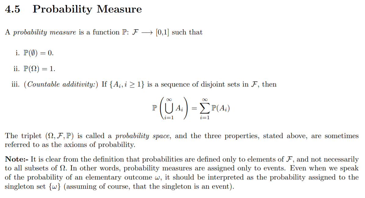
More precisely, the probability law assigns to every event a number
, called the probability of A , satisfying the following axioms.
- Nonnegativity
- Additivity
- Normalization
- [x] ### Properties of Probability Laws
There are many natural properties of a probability law which can be derived from the axioms.
We can use Venn diagrams for visualization and verification of various properties of probability laws.
And an intuitive reason of this is that Probability itself is a measure of set(sample space).
That means we can get disjoint sets and use the additivity and nonnegative property, this is consistent with the Venn diagrams, which can be viewed as a way to describe the element measure of sets.
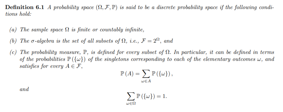
- [ ] ### Discrete Models
Sample space: a finite number of possible outcomes.
Discrete Probability Law:
- [ ] ### Continuous Models
Use the measure theory to build the model.
- [ ] ### Models and Reality
Stages of Probability Theory development.
1.3 Conditional Probability
- [ ] ### Introduction and Definition
In many cases, we may have already known some information about the outcomes. So the original probability law can’t be correspond with the new situation, thus we want to find a new probability law to rebuild our model taking the known facts into account.
And that is so called conditional probability. Conditional probability provides us with a way to reason about the outcome of an experiment based on the partial information.
In our beliefs, or intuitively speaking, what does it mean if you tell me the partial information such that event has already happened?
Caution! The information that event
happened means that the experiment is finished, and we are analyzing the result , and we have the partial information that
It means that we now stands in the new universe B, and we need to reset the probabilities of each event.
How can we do that? – By normalizing the original probability using .
Generalizing the argument , we get the definition:
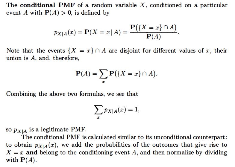
- [ ] ### Conditional Probabilities Specify a Probability Law
To check the three axioms.
(Because the conditional probability is constructed by our intuition, so we need to use the axioms to check whether it is a probability law.)
Conditional probabilities constitute a legitimate probability law, all general properties of probability laws remain valid.
- [ ] ### Using Conditional Probability for Modeling
When constructing probabilistic models for experiments that have a sequential character(physics process or logic sequence), it’s often natural and convenient to fist specify conditional probabilities and then use them to determine unconditional probabilities.
A useful rule for calculating various probabilities in conjunction with a tree-based sequential description of an experiment-------Multiplication Rule.
Example 1.9 Radar Detection
Example 1.11 graduate and undergraduate partition(for all the cases, the same logic sequential analysis)
Example 1.12 The Monty Hall Problem(the key is to choose sample space appropriately)
1.4 Total Probability Theorem and Bayes’ Rule
- [ ] ### Total Probability Theorem
Use the “divide-and-conquer” approach with a partition of the sample space.
Example 1.15 Alice taking probability class: the recursion relationship of total probability theorem can reduce a lot calculation compared with just using multiplication rule along the branch.
- [ ] ### Inference and Bayes’ Rule
Bayes’ rule is often used for inference. There are a number of “causes” that may result in a certain “effect”. We observe the effect, and we wish to infer the cause.
Example 1.16 Radar Detection 2.0
1.5 Independence
- [ ] ### Introduction and Definition
Conditional probability is used to capture the partial information that event
provides about event
. An interesting and important special case arises when the occurrence of B provides no such information and does not alter the probability that
has occurred.
Independence is often easy to grasp intuitively(distinct, noninteracting physical process) ,however it is not easily visualized in terms of the sample space.
Example 1.19(b)
- [ ] ### Conditional Independence
Since conditional probability is a legitimate probability law ,we can thus talk about independence of various events with respect to this conditional law.
Independence of two events and
with respect to the unconditional probability law does not imply conditional independence and vice versa.
Example 1.21 Biased coin
- [ ] ### Independence of a Collection of Events
Pairwise independence does not imply independence and the equality is not enough for independence.
Example 1.22/1.23
- [ ] ### Reliability
Divide the system into subsystems which consists of components that are connected either in series or in parallel.
- [ ] ### Independent Trials and the Binomial Probabilities
If an experiment involves a sequence of independent but identical stages, we say that we have a sequence of independent trials. In the special case where there are only two possible results at each stage, we say that we have a sequence of independent Bernoulli trials.
1.6 Counting
- [ ] ### The counting Principle
Consider a process that consists of r stages. Suppose that:
(a) There are possible results at the first stage.
(b)For every possible result at the first stage,there are possible results at the second stage.
© More generally, for any sequence of possible results at the first stages, there are
possible results at the
th stage. Then, the total number of possible results of the
stage process is
If the order of selection matters, the selection is called a permutation, and otherwise, it is called a combination. We will then discuss a more general type of counting, involving a partition of a collection of objects into multiple subsets.
- [ ] ###
-permutations
Example 1.29 CD-arranging problem
- [ ] ### Combinations
Counting arguments sometimes lead to formulas that are rather difficult to derive algebraically.
From the view of set and the view of combination formula to derive an equality involving $2^n \ and \ \tbinom{n}{r} $
Remember the picture of the relationship between permutation and combination.
Example 1.31 Choose a group leader
- [ ] ### Partitions
Combination can be viewed as a partition of the set in two, and now let’s consider partitions of the set into r disjoint subsets.
Using stage method, we can get the following formula:(Attention, are different, if
of them are the same, we need to divide the formula by
, this is in Problem 62)
After canceling we get:
This is called multinomial coefficient and is denoted by:
Example 1.32 TATTO rearrange problem
Example 1.33 graduate and undergraduate partition
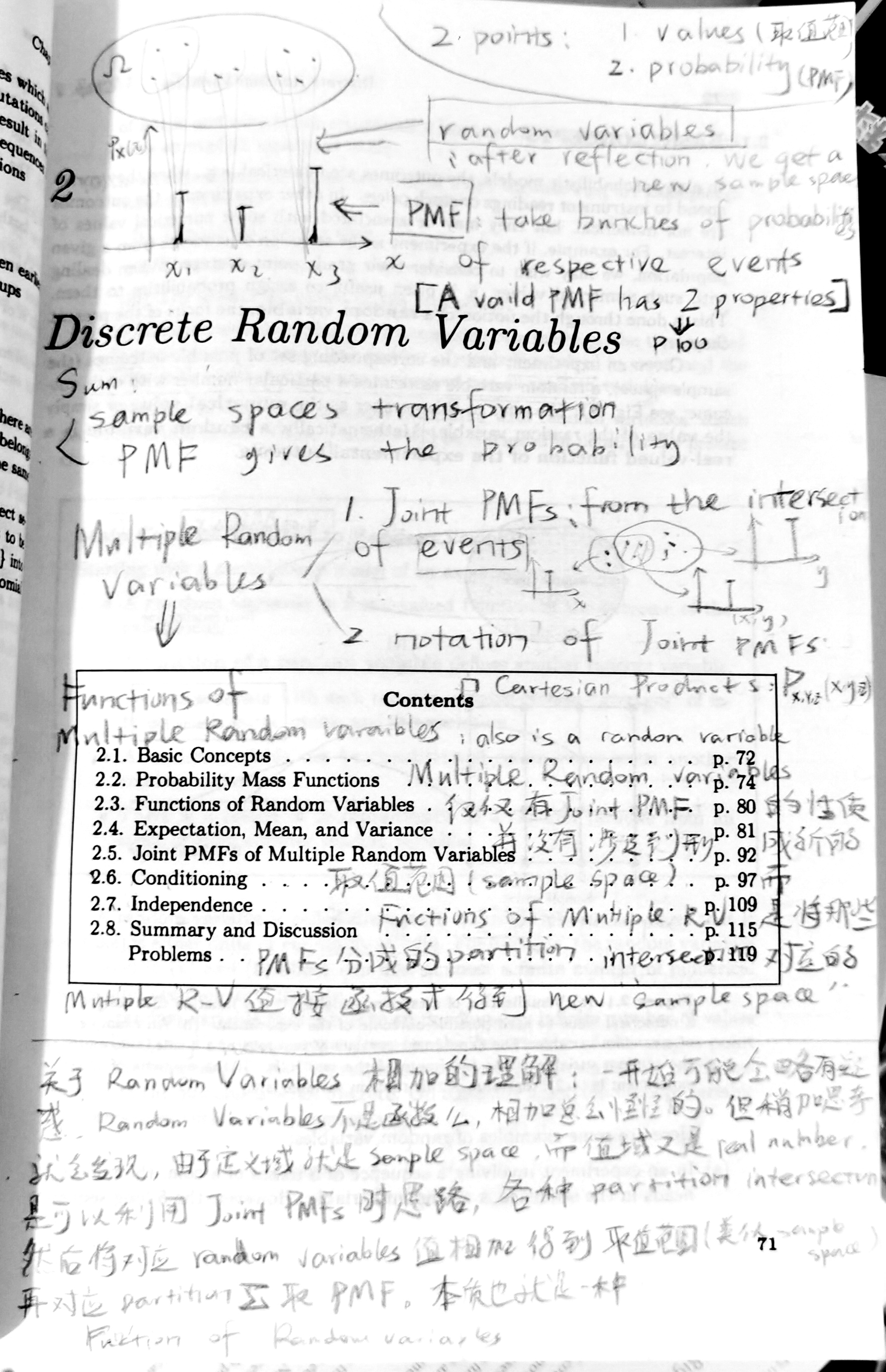
2. Discrete Random Variables
Overlook the Chapter
In this Chapter, we focus on discrete random variable. We first introduce some basic concepts. The concepts such as , the mean, and the variance describe in various degrees of detail the probabilistic character of a random variable. After that, we come to the
. It can be viewed as a measure on
since if the range of random variable chosen as a Borel set then the inverse image (correspond events) are also
algebra, it’s natural to assign probability to the value of random variable, which is the probability of the event
. Then we will learn some important random variables , also the functions of a random variable, whose
calculation is almost the same as the
of a single random variable.
For expectation, we will learn the intuitive diagram explaining expectation as the center, and the well-defined expectation, the expected value rule for functions of random variables, properties of mean(linear function). And also the variance.
For the experiment involving several random variables, we use the joint to describe the interdependence and the probability of any event that can be specified in terms of the random variable. And then we come to conditional and independence.
Condition on an event, condition on a random variable ,conditional expectation(total expectation theorem).
Independence of a random variable and an event, independence of random variables, and the property of expectation and variance under independence.
See the note
For random variables, there is a great explanation.
http://www.ee.iitm.ac.in/~krishnaj/EE5110_files/notes/lecture11_rvs.pdf
2.1 Basic Concepts
- [ ] ### Main Concepts Related to Random Variables
Starting with a probabilistic model of an experiment:
- Mathematically, a random variable is a real-valued function of the experimental outcome.
- A function of a random variable defines another random variable.
- We can associate with each random variable certain"averages"of interest, such as the mean and the variance.
- A random variable can be conditioned on an event or on another random variable.
- There is a notion of independence of a random variable from an event or from another random variable.
A random variable is called discrete if its range is either finite or countable infinite.
- [ ] ### Concepts Related to Discrete Random Variables
Starting with a probabilistic model of an experiment:
●A discrete random variable is a real-valued function of the outcome of the experiment that can take a finite or countably infinite number of values.
● A discrete random variable has an associated probability mass function(PMF),which gives the probability of each numerical value that the random variable can take.
●A function of a discrete random variable defines another discrete random variable, whose PMF can be obtained from the PMF of the original random variable.
2.2 Probability Mass Functions
- [ ] ### Definition
In particular, if is any possible value of
, the probability mass of
denoted
, is the probability of event
consisting of all outcomes that give rise to a value of
equal to
:
And as ranges over all possible values of
, the event
are disjoint and form a partition of the sample space.
- [ ] ### Calculation of the PMF of a Random Variable
For each possible value of
:
-
Collect all the possible outcomes that give rise to the event
.
-
Add their probabilities to obtain
.
2.3 Functions of Random Variables
If is a function of a random variable
, then
is also a random variable, since it provides a numerical value for each possible outcome. This is because every outcome in the sample space defines a numerical value
for
and hence also the numerical value
for Y. If
is discrete with
. then
is also discrete, and its
can be calculated using the
of
.In particular, to obtain
for any
, we add the probabilities of all values of
such that
:
Example 2.1 square function
2.4 Expectation, Mean, and Variance
- [ ] ### Expectation
The expectation of is a summary of the information provided by
in a single representative number.
We define the expected value (also called the expectation or the mean) of a random variable , with
, by
Expectation can be viewed as the center of gravity of the , remember the picture on page 83.
And the diagram is intuitively correspond to ‘Mass’ in the word PMF, also the word ‘moment’.
is called 2nd moment, because in physics, the form of
is the same as Momentum of Inertia
.
- [ ] ### Variance
The most important quantity associated with a random variable $ X$, other than the mean, is its , which is denoted by
and is defined as the expected value of the random variable
.
The variance provides a measure of dispersion of around its mean. Another measure of dispersion is the
of
with the same units, which is defined as the square root of the variance and is denoted by
:
- [ ] ### Expectation Value Rule for Functions of Random Variable
Let be a random variable with
, and let
be a function of
. Then, the expected value of the random variable $g( X) $is given by
Therefore, we just don’t need to find out the of
, the
of
is just enough.
- [ ] ### Properties of Mean and Variance
Mean and variance of a Linear Function of a Random Variable
Let be a random variable and let
where and
are given scalars. Then,
Unless is a linear function, it is not generally true that
is equal to
.
Example 2.4 Average Speed Versus Average time
Variance in Terms of Moments Expression
- [ ] ### Mean and Variance of Some Common Random Variables
See the notebook.
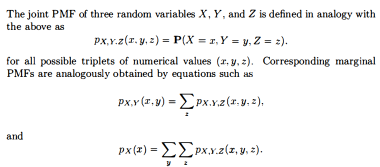
2.5 Joint PMFs of Multiple Random Variables
- [ ] ### Definition
Probability model often involve several random variables. All of these random variables are associated with the same experiment, sample space, and probability law, and their values may relate in interesting ways. This motivates us to consider probabilities of events involving simultaneously several random variables.
Consider two discrete random variables and
associated with the same experiment. The probabilities of the values that
and
can take are captured by the
of
and
, denoted
. In particular. if
is a pair of possible values of
and
, the probability mass of
is the probability of the event
:
The more precise notation is .
The joint determines the probability of any event that can be specified in terms of the random variables
and
.
And also formulas for the , with the reason.
We can use to derive marginal
from joint
.
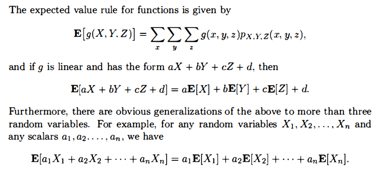
- [ ] ### Functions of Multiple Random Variables
When there are multiple random variables, it’s natural to generate new random variables by considering functions involving several of these random variables. In particular, a function of the random variables
and
defines another random variable. Its
can be calculated from the joint
according to
Furthermore, the expected value rule for functions naturally extends and take the form:
In the special case where is a linear function, with scalars
, we get
- [ ] ### More than Two Random Variables
Just natural extensions.
2.6 Conditioning
- [ ] ### Conditioning a Random Variable on an Event
Example 2.13 pass the test with trying maximum n times
- [ ] ### Conditioning a Random Variable on Another
Let and
be two random variables associated with the same experiment. If we know that the value of
is some particular
[with
], this provides partial knowledge about the value of
. This knowledge is captured by the $conditional\ PMF\ $
of
given
, which is defined by specializing the definition of
to events
of the form
.
Let us fix some with
and consider
as a function of
. This function is a valid
for
: it assigns nonnegative values to each possible
and these values add to 1. Furthermore this function of
has the same shape as
except that it is divided by
, which enforces the normalization property.
Example 2.15 the length of the message and the travel time of the message
- [ ] ### Conditional Expectation
Since the conditional is a legitimate
just over a new universe, conditional expectation seems to be reasonable.
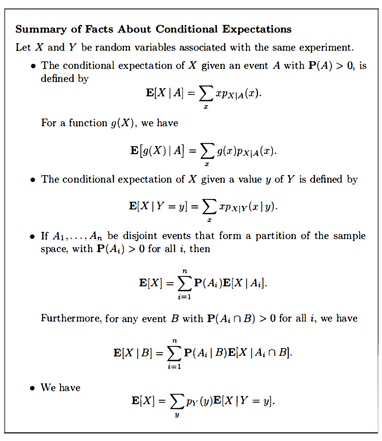
Total expectation theorem: the unconditional average and be obtained by averaging the conditional averages. That is, using a divide-and-conquer approach to calculate the unconditional expectation form the conditional expectation.
2.7 Independence
- [ ] ### Independence of a Random Variable from an Event
The idea is that knowing the occurrence of the conditioning event provides no new information on the value of the random variable, which is requiring that the two events and
be independent, for any choice
.
- [ ] ### Independence of Random Variables
We say that two random variable and
are independent if:
This is the same requiring that the two events and
be independent for every
and
.
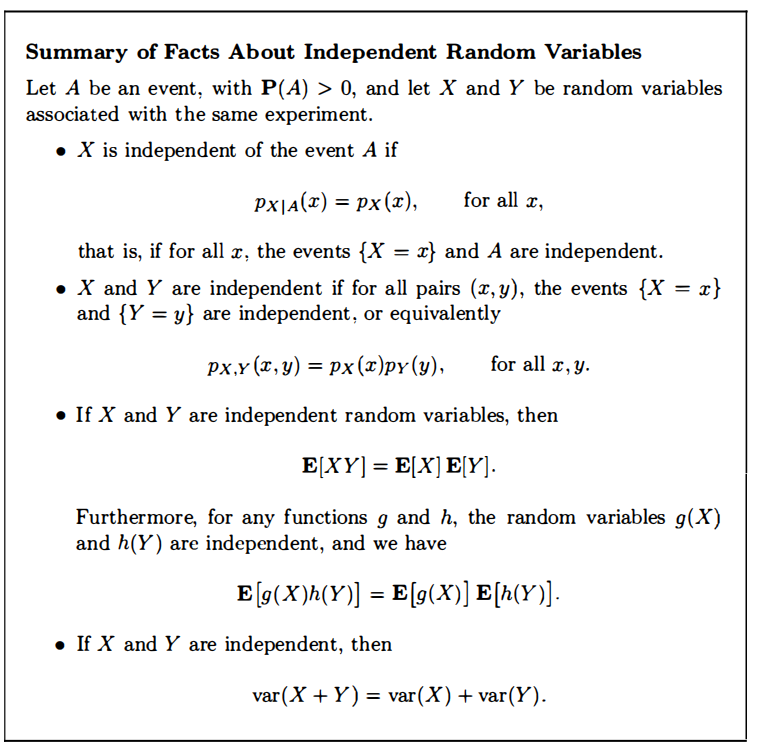
If and
are independent, then
- [ ] ### Independence of Several Random Variables
The preceding discussion extends naturally to the case of more than two random variables. For example. three random variables and
are said to be independent if
ps: The independence of several events seems to require the pairwise independence, but here we didn’t state that. In fact, the property of pairwise independence can be derived from the formula above easily.
- [ ] ### Variance of the Sum of Independent Random Variables
If are independent random variables, then:
3. General Random Variables
3.1 Continuous Random Variables and PDFs
- [ ] ### Continuous random Variable
A random variable is called continuous if there is a nonnegative function
, called the probability density function of
, or
for short, such that
for any .
To interpret the , note that for an interval
with very small length
, we have
so, we can view as the ‘probability mass per unit length’ near
.
- [ ] ### Expectation
The expected value or expectation or mean of a continuous random variable is defined by
and can also be interpreted as the ‘center of gravity’ of the .
If is a continuous random variable with given
, any real-valued function
of
is also a random variable(may be discrete or continuous). And the mean of
satisfies the expected value rule
3.2 Cumulative Distribution Functions
Loosely speaking, the ‘accumulates’ probability ‘up to’ the value
.
Any random variable associated with a given probability model has a , regardless of whether it is discrete or continuous. This is because
is always an event and therefore has a well-defined probability.
In what follows, any unambiguous specification of the probability of all events of the form , be it through a
or
, will be referred to as the probability law of the random variable
.
If is discrete and takes integer values, the
and the
can be obtained from each other by summing or differencing.
If is continuous, the
and the
can be obtained from each other by integration or differentiation.
Example 3.6 The Maximum of Several Random Variables
3.3 Normal Random Variables
A continuous random variable is said to be normal or Gaussian if it has a
of the form
The mean and the variance can be calculated to be
Normality is preserved by linear transformation.
- [ ] ### The Standard Normal Random Variable
A normal random variable with zero mean and unit variance is said to be standard normal. Its
is denoted by
:
More generally, we have
- [ ] ###
Calculation for a Normal Random Variable
For a normal random variable with mean
and variance
, we use a two-step procedure.
- “Standardize”
and divide by
to obtain a standard normal random variable
.
- Read the
Example 3.8 Signal Detection (+1,-1,signal and normal noise)
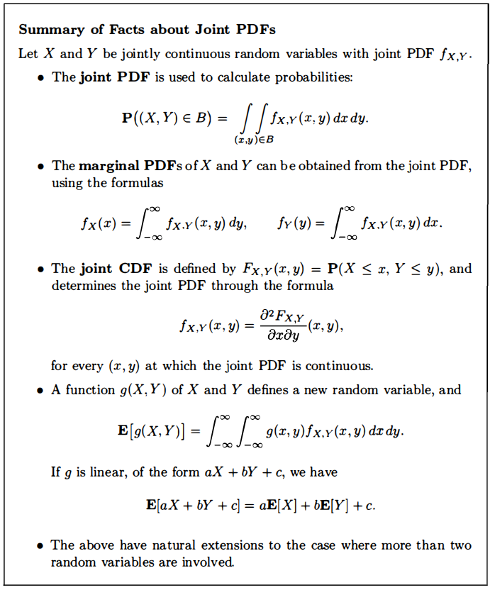
3.4 Joint PDFs of Multiple Random Variables
We say that two continuous random variables associated with the same experiment are jointly continuous and can be described in terms of a joint
if
is a nonnegative function that satisfies
We can view as the “probability per unit area” in the vicinity of
.
The joint contains all relevant probabilistic information on the random variables
and their dependencies.
Example 3.11 Buffoon’s Needle
- [ ] ### Joint
If and
are two random variables associated with the same experiment, we define their joint
by
Conversely, the can be recovered from the
by differentiating:
3.5 Conditioning
The various definitions and formulas parallel the ones for the discrete case, and their interpretation is similar, except for some subtleties that arise when we condition on an event of , which has zero probability.
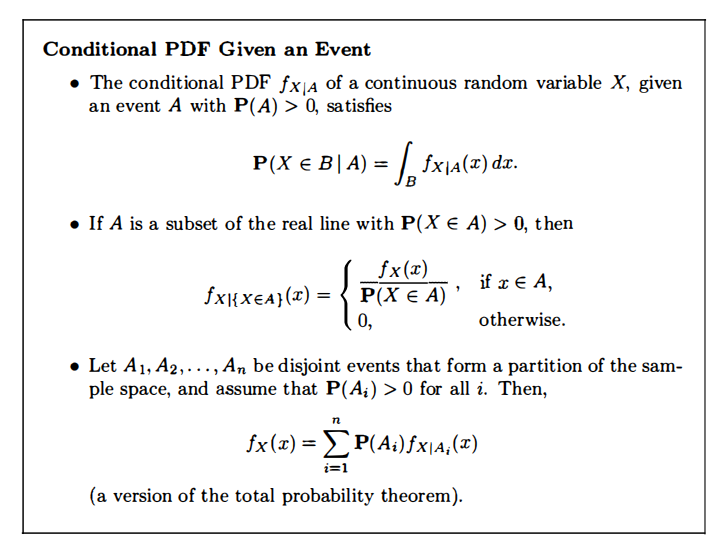
- [ ] ### Conditioning a Random Variable on an Event
Since we have the original idea towards condition, we just need to write the in terms of the continuous presentation.
Example 3.13 The Exponential Random Variable is Memoryless
- [ ] ### Conditioning one Random Variable on Another
Let and
be continuous random variables with joint
. For any
with
the conditional
of
given that
, is defined by
It is best to view as a fixed number and consider
as a function of the single variable
. Viewed as a function of
,
has the same shape as the joint
, because the denominator
does not depend on
.
3.6 The Continuous Bayes’ Rule
4. Further Topics on Random Variables
4.1 Derived Distributions
4.2 Covariance and Correlation
In the previous chapters, we just talked about the properties of functions of random variables using their joint distribution. But how about the random variables themselves? In another word, what information can we get from the multiple random variable? So now we are focused on the relationship between the random variables.
When dealing with multiple random variables, it is sometimes useful to use vector and matrix notations. This makes the formulas more compact and lets us use facts from linear algebra. When we have random variables
we can put them in a (column) vector
:
We call a random vector. Here
is an
dimensional vector because it consists of
random variables. We usually use bold capital letters such as
and
to represent a random vector. To show a possible value of a random vector we usually use bold lowercase letters such as x, y and z. Thus, we can write the
of the random vector
as
If the ’s are jointly continuous, the
of
can be written as
To calculate the expectation, first let’s see this, we can transfer the intuition of expectation to the multiple random variable case, that is the interpret the expectation as the center of gravity.(Consider probability as frequency, just think of doing experiments as the process of getting the points, so actually you are spreading out and filling the plain with different mass or density on each point, and when you do the experiment , the expectation is the weighted average of the all points.)
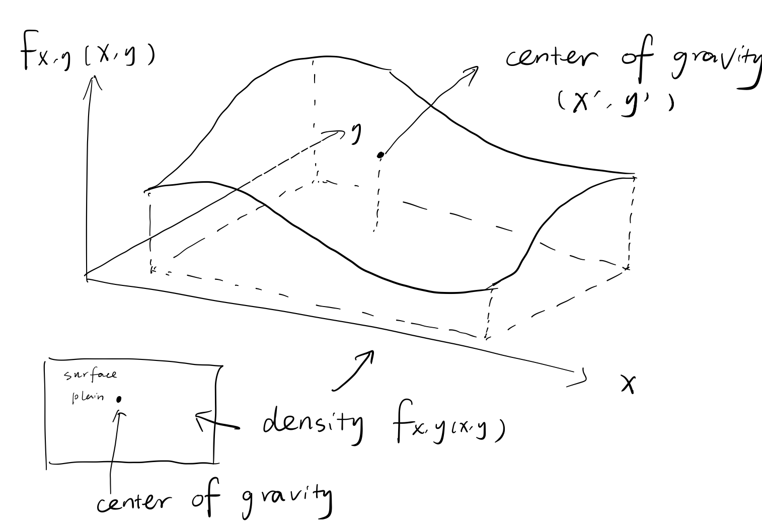
And using calculus, we can get the coordinate of center of gravity.
See here how to calculate: http://netedu.xauat.edu.cn/jpkc/netedu/jpkc/gdsx/homepage/5jxsd/52/092.htm
Actually , the coordinate is , a little amazing right?
The expected value vector or the mean vector of the random vector is defined as
4.3 Conditional Expectation and Variance Revisited
4.4 Transforms
4.5 Sum of a Random Number of Independent Random Variables
5. Limit Theorems
Overlook the Chapter
5.1 Markov and Chebyshev Inequalities
In this section, we derive some important inequalities. These inequalities use the mean and possibly the variance(Chebyshev) of a random variable to draw conclusions on the probabilities of certain events. They are primarily useful in situations where exact values or bounds for the mean and variance of a random variable are easily computable, but the distribution of
is either unavailable or hard to calculate.
- [ ] ### Markov Inequality
Loosely speaking(Or Intuitively speaking), it asserts that if a nonnegative random variable has a small mean, then the probability that it takes a large value must also be small.
Derivation(See the book)
But actually, the bounds provided by the Markov inequality can be quiet loose, so let’s come to a more powerful inequality ---- Chebyshev Inequality.
- [ ] ### Chebyshev Inequality
Loosely speaking, it asserts that if a random variable has small variance, then the probability that it takes a value far from its mean is also small.
ps: the random variable doesn’t need to be nonnegative.
Derivation(See the book)
The Chebyshev inequality tends to be more powerful than the Markov inequality(the bounds that it provides are more accurate), because it also uses information on the variance of .
Still, the mean and the variance of a random variable are only a rough summary of its properties, and we cannot expect the bounds to be close approximations of the exact probabilities.
Example 5.3: Upper Bounds in the Chebyshev Inequality
5.2 The Weak law of Large Numbers
The weak law of large numbers asserts that the sample mean of a large number of independent identically distributed(IID) random variables is very close to the true mean, with high probability.
Sample mean:
And the only assumption needed is that is well-defined.
Let be IID variables with mean
. For every
, we have
The weak law of large numbers states that for large , the bulk of the distribution of
is concentrated near
. In other words, the sample mean converges in probability to the true mean
.
Example 5.4 Probabilities and Frequencies
Example 5.5 Polling
5.3 Convergence in Probability
Convergence of a Deterministic Sequence
Convergence in Probability
Just read the definition on the book.
For convergence in probability, it’s also instructive to rephrase the above definition as follows: for every and for every
, there exists some
such that
If we refer to as accuracy level, and
as the confidence level, the definition takes the following intuitive form: for any given level of accuracy and confidence,
will be equal to
, within these levels of accuracy and confidence, provided that
is large enough.
The convergence to a number of a sequence
does not imply the convergence of
also to
.
Example 5.6 Min-sequence convergence
Example 5.7 Exponentially distributed over n sequence convergence
Example 5.8 The difference between convergence in probability and convergence in expectation
5.4 The Central Limit Theorem
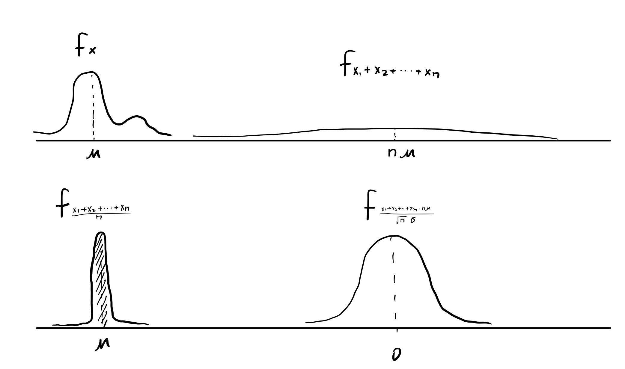
The distributions of and
are kind of extreme, an intermediate view is obtained by considering the deviation $S_n-n\mu $ of
from its mean
and scaling it by a factor proportional to
, which keeps the variance at a constant level.
The central limit theorem asserts that the distribution of this scaled random variable approaches a normal distribution.
Usefulness:
- Universal. Besides independence, and the implicit assumption that the mean and variance are finite, it places no other requirement on the distribution of
.
- Conceptual side. It indicates that the sum of a large number of independent random variable is approximately normal.
- Practical side. It provides accurate computational shortcut only requiring the knowledge of means and variances.
And it says that the of
converges to standard normal
, just a statement of
, not
or
. In fact, consider
is a discrete random variable, so mathematically speaking it has a
not a
. And in the case where
is not so large, the
looks very loose, which can’t be viewed as a approximation of standard normal
. That is why the
states that the
(not the
) of
converges to the standard normal
.
The following picture can be viewed as a intuitive explanation, where and
have been cooked up with the same mean and variance.
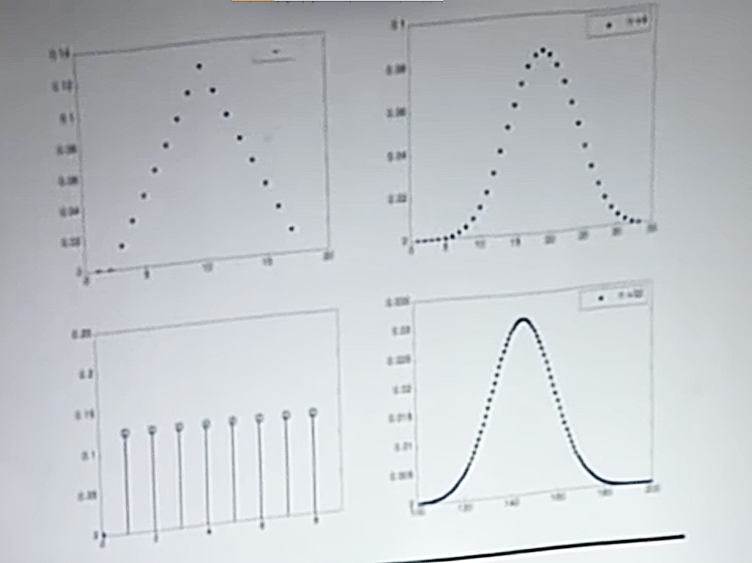
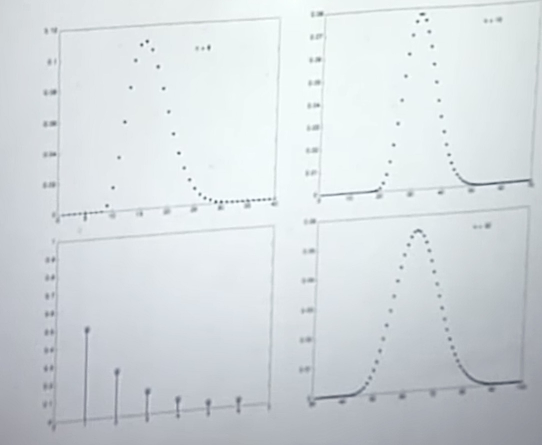
But actually, the shape of or
of
gets closer to the normal
as
increases. So, we can treat
as if normal. And also for
, which is just a linear transformation of
.
- [ ] ### Approximations Based on the Central Limit Theorem
The normal approximation is increasingly accurate as tends to infinity, but in practice we are generally faced with specific and finite values of
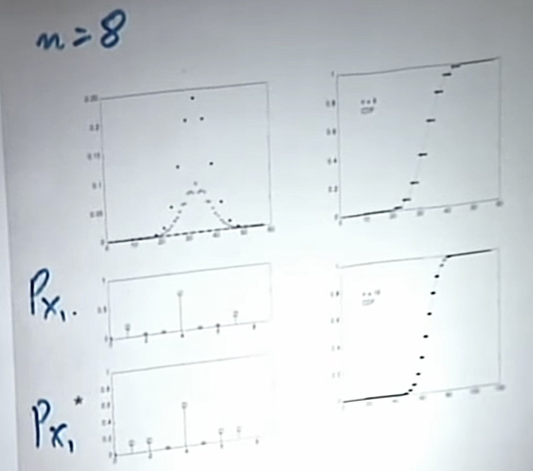
. And usually a small and appropriate number such as
can work well. It would be useful to know how large
should be before the approximation can be trusted, but there are no simple and general guidelines. Much depends on whether the distribution of the
is close to normal and, in particular, whether it is symmetric. 、
Calculation method
Since the of
can be viewed as a approximation of standard normal variable
, it can be viewed as if normal. And
and
can also be viewed as if normal. So, it comes back to the case of calculating the probability of normal distributed events. Just do the linear transformations on
and
to get the form of
, and use the approximation to transform the original problem to a standard normal distribution problem. The derivation (given
and to find the probability) and the inverse problem (given the probability and to find the appropriate
) is just also the same as the standard normal case.
Example 5.10 Machine processes parts in a given time
Example 5.11 Polling
- [ ] ### De Moivre-Laplace Approximation to the Binomial
A binomial random variable with parameter
and
can be viewed as the sum of
independent Bernoulli random variable
, with common parameter
.
We can use the approximation suggested by the to provide an approximation for the probability of the events
, where
and
are given integers,
But since the event is the same as
, it’s quiet reasonable to think of a nicer approximation. And it turns out that a more accurate approximation may be possible if we replace
and
by
and
, respectively.
In fact, we can use this idea to even calculate the individual probabilities. When
is close to 1/2, in which case the
of the
is symmetric,the above formula yields a very good approximation for
as low as 40 or 50. When
is near 1 or near 0. the quality of the approximation drops. and a larger value of
is needed to maintain the same accuracy.
Although, the is a statement of
, and it does not tell you what to do to approximate
itself, but in the Binomial case
can also give a good approximation on
.
- [ ] ### Paradox of CLT
Consider a Poisson process that runs over a unit interval and where the arrival rate is equal to 1. And now, divide it into little pieces as the picture below:
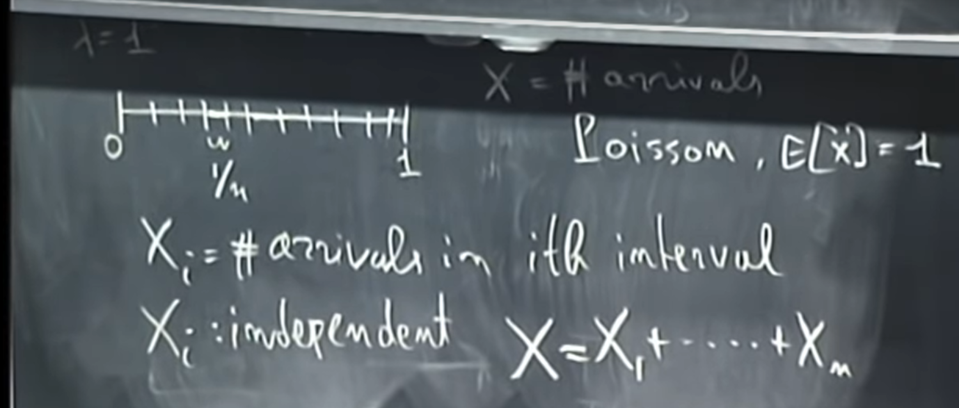
It seems that should follow a normal distribution, but
just has the Poisson distribution. So what’s wrong?
In fact, the implicit requirement of is that
should be fixed distributed. But
in the above case does change when changing the size
.
- [ ] ### The difference between Estimate using Poisson and CLT
5.5 The Strong law of Large Numbers
- [ ] ### a