Hi! This is zxr’s note of 6.034-artificial intelligence.😊

In general, it’s the record of lecture notes and zxr thinkings.

So, usually, i write the structure of lessons and inspiring ideas on paper when i watch the course. And later, i summarize them and generate the notes you see.

course and mega link:

6.034-course and 6.034-maga

zxr write most of the notes on paper, so this article is just like the supplement. Maybe zxr will scan and upload the paper note later. And i do recommend to read the textbook, because almost every concept proposed in class is explained in detail in the book.

1. Introduction and scope

What is artificial intelligence?

For representations, the professor gave the example of cycle rolling and the Fox、Goose、Grain、Farmer problem.

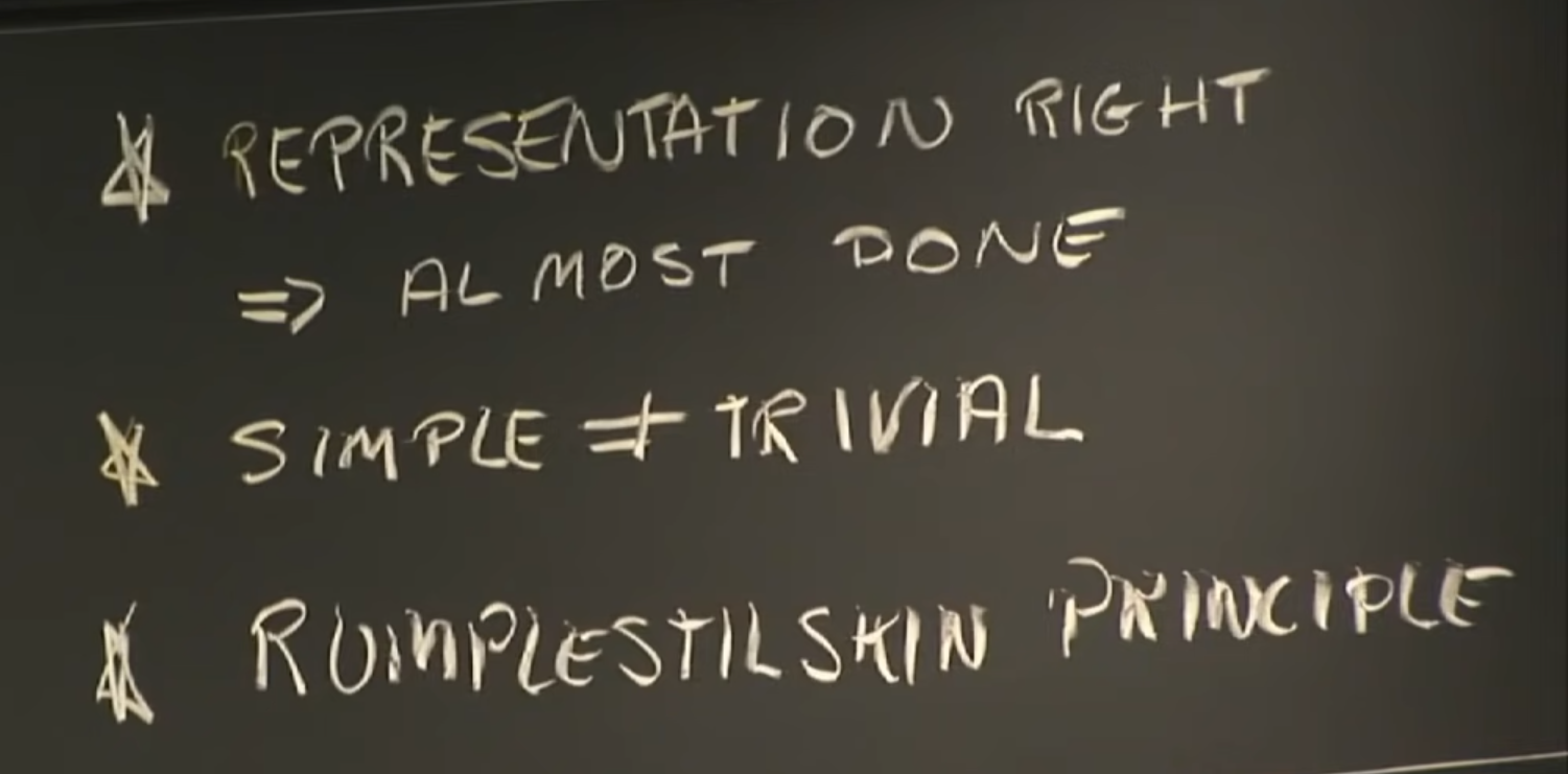
Rumpelstiltskin principle : Once you can name something, you get power over it.

General ideas

The history of AI.

species

The development of humans. What makes us different from chimpanzees?

Africa

2. Reasoning

Goal trees and Problem solving

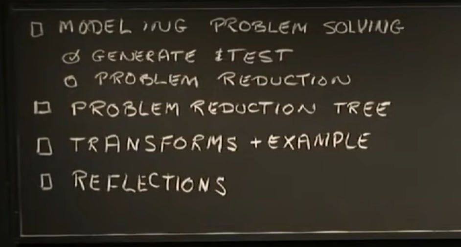
Introduction to problem solving model

So today we’re going to be modeling a little bit of human problem solving, the kind that is required when you do

symbolic integration. Now, you all learned how to do that. You may not be able to do that particular problem

anymore, but you all learned how to integrate in high school 1801, or something like that. The question is, how did

you do it, and is the problem solving technique that we are trying to model by building a program that does

symbolic integration, is that a common kind of description of what people do when they solve problems.

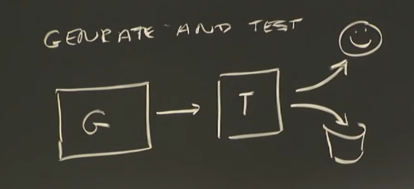
So the answer to the question is, yes. The kind of problem solving you’ll see today is like generating tests, which

you saw last time. It’s a very common kind of problem solving that we all engage in, that we all engage in without

thinking about it, and without having a name for it.

But once we get a name for it, we’ll get power over it. And then we’ll be able to deploy it, and it will become a skill.

We’ll not just witness it, we’ll not just understand it, we’ll use it instinctively, as a skill.

The whole process

So far, all we’ve done is talk about the safe transformations, but now we know that if

we’re not done, we need to find a problem to work on using that depth of functional composition business. And

then after that we apply heuristic transformation.

And the way Slagle designed his program is, he found just one problem to work on, did one transformation, then

went back around the loop. Because these heuristic transformations are a little harder to apply than the safe ones.

So I’ll given you an accurate portrayal of what this program did, except for one thing. Which I would like, now, to

go back and patch up. And that thing is over here. What to do with something like this. Well we got to that in a

board that’s disappeared, but when we tried to deal with this, we had to find a heuristic transformation.

And when we decided to work on this, it must have been the case that this was the simplest problem at a leaf

node that has not yet been solved.

So what’s the functional composition depth of this? It’s 3. Back over here, we have something that has a depth of

functional composition of 2. So when the program actually ran on this particular problem, it stopped a few inches

short of the finish line, And went back and screwed around with that other problem for a little bit, before it gave up

and came back here.

So it’s always looking across the whole tree, the leaves of the tree. Whenever it has to find a place to work on with

the heuristic transformation, it happened to look at all the leaves of the tree that had not yet been dealt with, tried

to find the easiest one, and that could involve a lot of backing up and starting over on a branch of the tree that it

had previously ignored. A small detail, not a particularly important one.

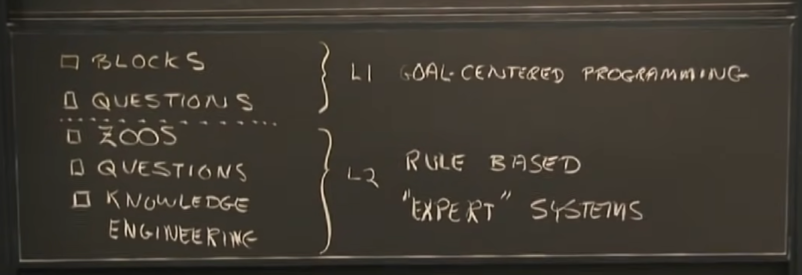
Goal trees and Rule-Based Expert Systems

But there’s a very important characteristic of this system in both backward and forward mode, and that is that this

thing is a deduction system.

That’s because it’s working with facts to produce new facts.

When you have a deduction system, you can never take anything away.

But these rule-based systems are also used in another mode, where it’s possible to take something away.

See, in fact world, in deduction world, you’re talking about proving things.

And once you prove something is true, it can’t be false.

If it is, you’ve got a contradiction in your system.

But if you think of this as a programming language, if you think of using rules as a programming language, then

you can think of arranging it so these rules add or subtract from the database.

In fact, I’ve listed this as a gold star idea having to do with engineering yourself because all of these things that

you can do for knowledge engineering are things you can do when you learn a new subject yourself.

Because essentially, you’re making yourself into an expert system when you’re learning circuit theory or

electromagnetism or something of that sort.

You’re saying to yourself, well, let’s look at some specific cases.

Well, what are the vocabulary items here that tell me why this problem is different from that problem?

Oh, this is a cylinder instead of a sphere.

Or you’re working with a problem set, and you discover you can’t work with the problem, and you need to get

another chunk of knowledge that makes it possible for you to do it.

So this sort of thing, which you think of primarily as a mechanism, heuristics for doing knowledge engineering, are

also mechanisms for making yourself smarter.

So that concludes what I want to talk with you about today.

But the bottom line is, that if you build a rule-based expert system, it can answer questions about its own behavior.

If you build a program that’s centered on goals, it can answer questions about its own behavior.

If you build an integration program, it can answer questions about its own behavior.

And if you want to build one of these systems, and you need to extract knowledge from an expert, you need to approach it with these kinds of heuristics because the expert won’t think what to tell you unless you elicit that

information by specific cases, by asking questions about differences, and by ultimately doing some experiments to

see where your program is correct.

3. Search

Search for a good solution

Search for a best solution

With your eye, you can find a good path.

But you can’t find the best possible path.

Today, what we’re doing is probably not modeling any obvious property of what we have inside our heads.

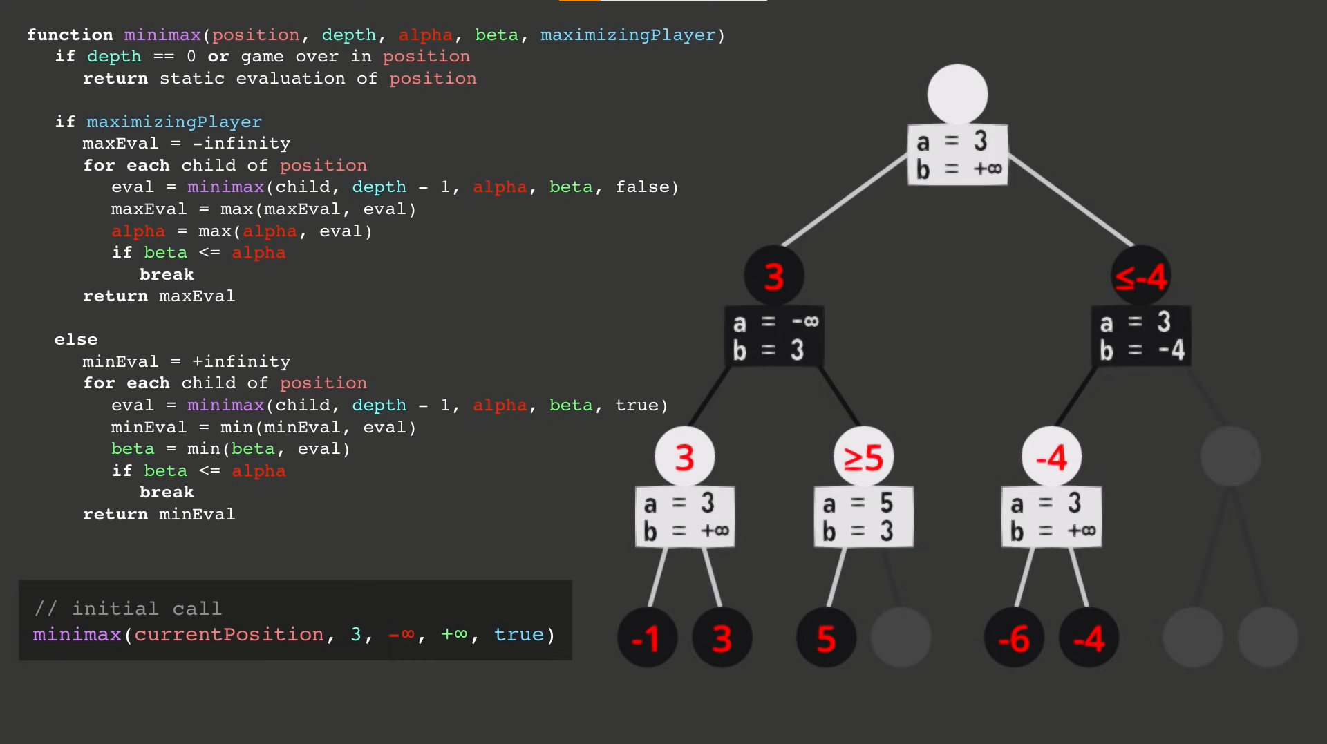
Search in Game

Use the idea of depth-first, just translate the simulation process into the programming language. We use and to give a rough range of each node value, and this can be presented by the 2 parameters and . When it comes to the conflict situation where , we can prune the branch. And for one node, its or is got by the value of its child nodes, if the child . The key is that use the parent(maxim for example) node’s to check its right branch child nodes’ to prune the branch.

4. Constrains

Constraint Satisfaction

Constraint satisfaction algorithms that we have learned about:

DFS with Backtracking ( BT ). No constraint checks are propagated [“Assignments only”]. One variable is
assigned a single value at a time, and then the next variable, and the next, etc. Check to see if the current partial
solution violates any constraint. Whenever this check produces a zero-value domain, backup occurs.
DFS with Backtracking + Forward-checking. A variable is assigned a unique value, and then only its neighbors
are checked to see if their values are consistent with this assignment. That is: assume the current partial assignment,
apply constraints and reduce domain of neighboring variables. [“ Check neighbors of current variable only”].
DFS with Backtracking + Forward-checking + propagation through singleton domains. If during forward
checking you reduce a domain to size 1 (singleton domain), then assume the assignment of the singleton domain
and repeat forward checking from this variable. (Note that reduction to a singleton domain and repeated forward
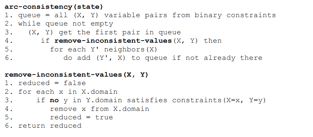
checking might lead to yet another singleton domain in some cases.)
DFS with Backtracking + Forward checking + propagation through reduced domains (this is also known as:
Arc-consistency, AC-2, since it ensures that all *pairs* of variables have consistent values). Constraints are
propagated through all reduced domains of variable values, possibly beyond immediate neighbors of current
variable, until closure. [“Propagate through reduced domains”; also called “Waltz labeling”]
1. Map coloring – comparing Backtracking (BT) with Forward-checking+propagation through singleton domains.

Constraint Types
- Unary Constraints – constraint on single variables (often used to reduce the initial domain)
- Binary Constraints – constraints on two variables , *C* ( *X, Y* )
- n-ary Constraints – constraints involving n variables. Any n-ary variables n > 2
(Can always be expressed in terms of Binary constraints + Auxiliary variables

Search Algorithm types:

DFS w/ BT + basic constraint checking: Check current partial solution see if you violated any constraint.
DFS w/ BT + forward checking: Assume the current partial assignment, apply constraints and reduce
domain of other variables.
DFS w/ BT + forward checking + propagation through singleton domains: If during forward checking, you
reduce a domain to size 1 (singleton domain), then assume the assignment of singleton domain, repeat
forward checking from singleton variable.
DFS w/ BT with propagation through reduced domains (AC-2): see below.

Note: You can replace DFS with Best-first Search or Beam-search if variable assignments have “scores,” or if you
are interested in the best assignments.

Definitions.

k- consistency. If you set values for k – 1 variables, then the k th variable can still have some non-zero domain.
2 - consistency = arc-consistency.
o For all variable pairs (X, Y)
o for any settings of X there is an assignment available for Y
1 - consistency = node-consistency
o For all variables there is some assignment available.
Forward Checking is only checking consistency of the current variable with all neighbors.
Arc-consistency = propagation through reduced domains
Arc-consistency ensures consistency is maintained for all pairs of variables, also known as AC- 2
Variable domain (VD) table – bookkeeping for what values are allowed for each variable.

Variable Selection Strategies :

Minimum Remaining Values Heuristic (MRV): Pick the variable with the smallest domain to start.
Degree Heuristic – usually the tie breaker after running MRV: When domains sizes are same (for all
variables), choose the variable with the most constraints on other variables (greatest number of edges in
the constraint graph)

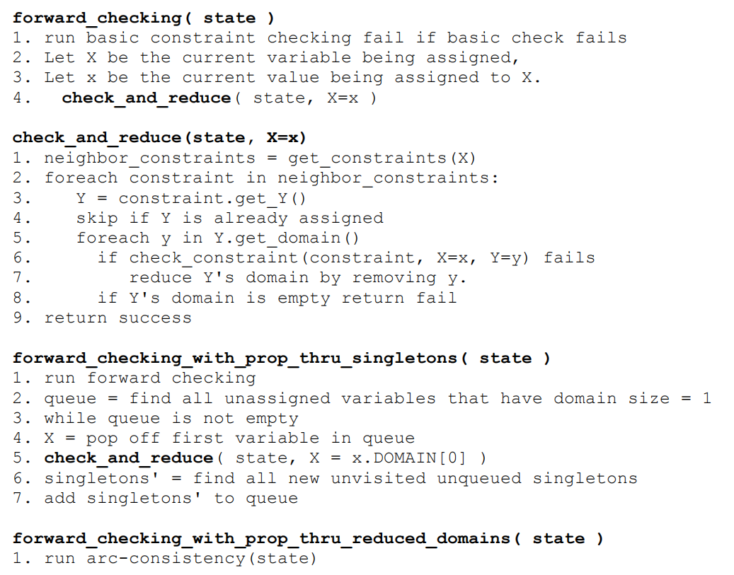
Forward Checking Pseudo Code:
Assume all constraints are Binary on variables X, and Y.
constraint.get_X gives the X variable
constraint.get_Y gives the Y variable
X.domain gives the current domain of variable X.